Generalized Marginal Risk

(1)

Munich Personal RePEc Archive

Generalized Marginal Risk

Keel, Simon and Ardia, David

aeris CAPITAL AG

11 September 2009

(2)

Simon Keel aeris CAPITAL AG

Switzerland

Email:[email protected]

Phone: +41 (55)5 111 222

David Ardia aeris CAPITAL AG

Switzerland

Email:[email protected]

Phone: +41 (55)5 111 222

Abstract

An important aspect of portfolio risk management is the analysis of the overall risk with respect to the assets’ allocations. Marginal risk is the traditional tool, however, this metric is only meaningful when a position is levered or when the proceeds from the sale of a position are put in the cash account. This paper proposes an extension of the traditional marginal risk approach as a means of overcoming this deficiency. The new concept addresses situations where the change in a position results in changes to other positions as well. An illustration is provided for synthetic and real-world portfolios.

Keywords: Marginal risk, component risk, Value-at-Risk, expected shortfall, elliptical distri-bution.

(3)

Abstract

An important aspect of portfolio risk management is the analysis of the overall risk with respect to the assets’ allocations. Marginal risk is the traditional tool, however, this metric is only meaningful when a position is levered or when the proceeds from the sale of a position are put in the cash account. This paper proposes an extension of the traditional marginal risk approach as a means of overcoming this deficiency. The new concept addresses situations where the change in a position results in changes to other positions as well. An illustration is provided for synthetic and real-world portfolios.

Keywords: Marginal risk, component risk, Value-at-Risk, expected shortfall, elliptical distri-bution

(4)

1. Introduction

Portfolio risk management requires assessing the aggregated risk of a portfolio. Nowadays, the industry standards for such risk measures are the Value-at-Risk (VaR) and the expected shortfall (ES). A large stream of research has been devoted to their unbiased and efficient estimation; see, e.g.,Duffie and Pan(1997),Jorion(2001) andGourieroux and Jasiak(2009). However, as mentioned byLitterman (1996a), aggregated risk measures are useful for moni-toring risk but they do not provide much guidance for practical risk management.

In order to manage the risks of a portfolio effectively, the risk impact of new trades and/or reallocations within the portfolio must be assessed. Moreover, the sources of risk in the current portfolio need to be identified. Generally speaking, the aim of the portfolio risk analysis is to gain insight through the sensitivity of the aggregated risk with respect to the portfolio holdings as well as the attribution of the portfolio risk to the underlying components through decomposition. In the financial literature, these concepts are referred to asmarginal risk and

component risk, respectively. For an introduction, the reader is referred toLitterman(1996a, 1997a,b) and Jorion(2001).

The marginal risk aims at measuring how investment decisions affect the risk profile of the portfolio. Mathematically, this is simply the gradient of the portfolio risk measure with respect to the allocation weights. It is therefore defined as the linear approximation of the change in the portfolio risk when a position is altered while all other positions remain the same. This sensitivity measure is precise for infinitesimal changes; however these are rarely the case in practice. A portfolio manager would typically relate this marginal change with the expected return on the various assets in the portfolio in order to increase its risk-adjusted performance. The risks of portfolio holdings are generally not additive with respect to the overall portfo-lio risk. While this is desirable from a diversification viewpoint, this does not allow for a straightforward decomposition of risk in the portfolio. The component risk is an attempt at measuring the proportion of the portfolio risk that can be attributed to each of the individual positions. With this metric, a portfolio manager is able to target the most significant sources of risk; the so-calledhot spots (seeLitterman 1996a). The mathematical construction of com-ponent risk is based on the Euler decomposition of positive homogeneous functions and was first used by Litterman (1996a) for decomposing the standard deviation of a portfolio. Gar-man(1996,1997) used this approach for decomposing the portfolio VaR. This mathematical decomposition expresses the portfolio risk as a sum of each position weight times the marginal risk of the position. The marginal risk is therefore a building block of the component risk. While the component risk provides a way to decompose the portfolio risk, we stress that it needs to be interpreted carefully. Indeed, a pure mathematical decomposition of the portfolio risk measure does not guarantee that the results are meaningful in the financial sense. See Sharpe(2002) for further details.

(5)

4 Generalized Marginal Risk

This paper proposes a novel approach to tackle this issue, which we namegeneralized marginal risk. As for the traditional marginal risk, the new concept allows a portfolio manager to measure the sensitivity of the portfolio to new marginal allocations. However, it ensures that potential effects on the other positions are correctly taken into account. This therefore helps analyzing the risk impact under more general and realistic scenarios. Moreover, we show that the generalized marginal risk and its traditional counterpart are directly related. Therefore, once the marginal risks have been estimated, a portfolio manager can run a generalized sensitivity analysis in a straightforward manner. We illustrate the usefulness of the new metric with a synthetic and a real-world portfolio within the elliptical framework.

The paper proceeds as follows. Section 2 briefly reviews the marginal and component risk. Section3 introduces the new concept of generalized marginal risk. Section 4 illustrates the usefulness of the new metric. Section5 concludes.

2. Marginal Risk

First, let us introduce some notation. We assume that the portfolio is composed of n assets whose arithmetic returns are given by the (n×1) random vectorX = (X. 1, . . . , Xn)′and whose

allocation weights are collected into the (n×1) vector w= (w. 1, . . . , wn)′. Additionally, the

portfolio consists of a cash account with weight w0 = 1. −Pni₌₁wi which we assume as

risk-free. The portfolio is levered when w0 < 0. We denote the portfolio return by P(w) to emphasize the fact that it is a function ofw. For underlying arithmetic returns, this function is linear, i.e., P(w) =. w′_X_{. Finally, we denote the risk measure of the portfolio return by}

ρ(w)=. ρ{P(w)}where the notation again emphasizes the fact that it is a function ofw. We assume that ρ(w) is at least once differentiable.

Definition 2.1 _{(Marginal risk)}. _{For the risk measure} _{ρ, the marginal risk of the} _{ith asset}

in the portfolio, denoted by ρmi , is defined as the change in the portfolio risk measure for an

infinitesimal change in the allocation to the ith asset. Formally, this is the derivative of ρ(w) with respect to wi:

ρmi (w)

. = ∂

∂wi

ρ(w). (1)

For convenience, the n marginal risks of the portfolio are collected into the (n×1) vector ρm= (ρ. m₁ , . . . , ρmn)′;ρmis the gradient of ρ(w).

In some cases, the marginal risks ρmi can be computed explicitly (see Section 4.1). If a

parametric model is available for the distribution of P(w), the derivatives with respect to the holdings are either obtained in closed-form or can be computed efficiently by numerical methods. For Monte Carlo approaches (i.e., when the portfolio return distribution is obtained by simulation), the so calledbrute force orbefore and after approach described inDowd(1998) can be used. In this case, a marginal ∆w is added to each wi iteratively, the risk of the new

(6)

as the VaR and ES; see, e.g., McNeil, Frey, and Embrechts(2005). Under this condition, the risk measure can be decomposed as

ρ(w) =

n

X

i=1 wi

∂ ∂wi

ρ(w) =

n

X

i=1

wiρmi (w) = n

X

i=1

ρci(w), (2)

where the termρci

.

=wiρmi (w) is defined as the component risk of theith asset in the portfolio.

As we can see in (2), the marginal risk is a building block of the component risk. We can therefore interpret ρci as the linear approximation of the risk impact of theith allocation if

we remove the corresponding asset in the portfolio and put the proceeds in the cash account. On the other hand, if a new asset is included in the portfolio, the component risk approxi-mates the risk impact of the new position in the augmented portfolio; this is known as the

incremental risk of the new asset. In both cases, the larger the position size the worse the linear approximation.

It is important to emphasize two important limitations of the marginal and component risk. First, both concepts are based on a marginal argument, and this must be kept in mind when interpreting the measures. Indeed, consider the case where a particular position accounts for half the risk according to the component risk. This implies that a small percentage increase in that position will increase the portfolio risk as much as a combined similar percentage increase in all other positions. However, it does not imply that eliminating that position entirely will reduce risk by half. Indeed, as the size of the position of a contributor to risk is reduced, the marginal contribution of that position to risk will be reduced as well (Litterman 1996b, p.29). Second, the marginal risk is the linear approximation of the risk impact of leveraging the corresponding position in the portfolio. Indeed, the gradient is the linear approximation of the change in the portfolio risk when a position is altered while all others remain constant. In order to illustrate this point, let us assume thatw0 = 0 (i.e., Pni₌₁wi= 1), which is the case

for a fully funded portfolio with an empty cash account. The marginal risk does introduce leverage for this case since altering a position and leaving all others constant implies w0 6= 0. In the case where we are interested in the portfolio risk impact for an increase in size of a certain position we obviously have w₀ <0, even for an infinitesimal increase of any portfolio weight.

3. Generalized Marginal Risk

In practice, it is also important to consider scenarios where the change in a position results in the change of other positions as well. This is typically the case when there are capital in-and outflows in the portfolio since all percentage allocations change in this situation. Another example is when the increase in a position is funded by the reduction of other positions. In this case, the weights of other components must be rescaled accordingly when computing the sensitivity of the portfolio risk. The concept of generalized marginal risk aims at dealing with these scenarios.

Definition 3.1 _{(Generalized marginal risk)}. _{Let us denote by} _w_e_i_(δ)₌. _w₊_δf_i_{(w) the new}

allocation vector of the portfolio after allocating an additionalδ percent of the investor’s total wealth to the ith asset. The function fi : Rn → Rn describes how an additional δ percent

(7)

scheme. The generalized marginal risk of the ith asset in the portfolio, denoted by ρgmi , is

defined as the derivative ofρ(wei(δ)) with respect to δ, evaluated atδ= 0:

ρgmi (w)

. = ∂

∂δρ(wei(δ))

_δ

=0

=

∂

∂wρ(wei(δ))

′ _δ

=0

· ∂wei(δ)

∂δ

_δ

=0 =ρm(w)′_f_i_(w)_.

(3)

Then generalized marginal risks of the portfolio are collected into the (n×1) vector ρgm=. (ρgm₁ , . . . , ρgmn )′ for convenience. Expression (3) shows the direct relationship between the

marginal and the generalized marginal risk. Therefore, once the marginal risks of the positions have been computed, a portfolio manager can run a generalized sensitivity analysis in a straightforward manner. Note that we use the chain rule in (3) but the directional derivative ofρ in direction of fi(w) leads to the same result.

In order to gain insight on this new concept, we assume that an investor has an additional δ to invest in the portfolio, expressed as a percentage of the total wealth (i.e., the current wealth plus the additional wealth). If the investor adds this capacity to theith asset, the new allocation vector reads

e

wi(δ) =w(1−δ) +δei

=w+δ(ei−w)

where ei denotes the ith (n×1) basis vector. The term w(1−δ) represents the effect of

adding δ amount of new capital to the portfolio while the term δei reflects the fact that the

ith position is increased byδ. In this case fi(w) = (ei−w) and using (3) yields

ρgmi (w) =ρm(w)′(ei−w).

By stacking n times the weight vectors in a (n×n) matrix W = [w. · · ·w], we can express the (n×1) vector of generalized marginal risks as

ρgm(w) =ρm(w)′_(I_n₋_W₎_, ₍₄₎

whereIn denotes the (n×n) identity matrix.

Another example arises when a portfolio manager is interested in changes of the portfolio risk when reallocating capital within the portfolio. For instance, consider the case where the δ increase in theith position is financed through an equal reduction of all other positions. After this adjustment, the allocation vector reads

e

wi(δ)=. w+δλi,

where λi denotes a (n×1) vector whose components are all equal to −_n1

−1 except the ith

position which equals one. In this case fi(w) =λi and using (3) yields

(8)

In vector form we obtain

ρgm(w) =ρm(w)′

n n−1In−

1 n−1Jn

, (5)

whereJn denotes the (n×n) matrix of ones. Obviously we do not necessarily need to finance

the reallocation by reducing all other positions proportionally. By modifying the vectorλi,

a portfolio manager has full control on how assets are to be shifted within the portfolio. For instance, the investor could look for the directionλk which reduces risk the most in order to

find the most suitable portfolio adjustments to increase thekth position.

As a last example, consider the increase in the ith position financed through leverage. The allocation vector reads

e

wi(δ)=. w+δei.

In this casefi(w) =ei and using (3) we obtainρgmi (w) =ρmi (w). Therefore, the generalized

marginal risk for a scenario of leverage equals the traditional marginal risk.

Finally, note that if we multiply the generalized marginal risk with the corresponding asset weight we obtain a linear approximation of the change in the portfolio risk if a position is closed and the proceeds are treated as defined through the functionfi(w). Contrary to the

marginal risk, the decomposition of the portfolio risk in terms of generalized marginal risks is not possible sincePni₌₁wiρgmi 6=ρ in general. We could consider the portfolio risk ρ as a

function of wand δ, and then perform the Euler decomposition. Since δ equals zero for the current portfolio we would simply obtain the traditional component risk. Alternatively, the productswiρgmi could be rescaled in order to sum up to the portfolio risk. However, we prefer

to have a unique decomposition of risk with a meaningful financial interpretation.

4. Illustrations

We now illustrate the differences between the marginal and the generalized marginal risk within the elliptical framework. First, we consider a synthetic portfolio of two assets whose returns are modeled by a multivariate Gaussian distribution. We consider different weights in order to see the extent of the discrepancy between the marginal and generalized marginal VaR at the 95% confidence level in different correlation-volatility scenarios. For the generalized marginal risk, we investigate the case of reallocating capital equally within the portfolio. Second, we extend the illustration to a real-world equity portfolio, whose asset returns are modeled by a multivariate Student-tdistribution. In this case, we compare the marginal and generalized marginal ES at the 95% confidence level. We investigate the cases of capital in-and outflows as well as reallocating capital within the portfolio.

4.1. Elliptical Framework

(9)

elliptical. Popular examples are portfolios of equities. The reader is referred toMcNeilet al.

(2005) for an excellent introduction on elliptical distributions.

A (n×1) random vectorX of asset returns which follows an elliptical distribution is denoted by X ∼En(µ,Σ, ψ), where µis a (n×1) location vector, Σis a (n×n) dispersion matrix

and ψ(·) is the characteristic generator. Since the class is closed under affine transformations, the distribution of the linear portfolio P(w) =. w′_X _{is obtained in closed-form as} _P_(w) _∼

E1(w′µ,w′Σw, ψ).

In the sequel, we will focus on the VaR and ES as the risk measures of interest. Both risk measures are obtained in a straightforward manner within the elliptical framework. Indeed, sinceP(w)∼E₁(w′_µ,_w′Σ_{w, ψ) we have}P(w) =w′_µ_{+ (w}′Σ_w)12 Z, whereZ ∼E₁(0,1, ψ).

Using the latter expression, we obtain closed-form expressions for the VaR and ES as

ρ(w) =ρnw′_µ₊ _w′_Σ_w12_Z

o

=w′_µ₊_ρ_{_Z_} _w′_Σ_w12 _,

(6)

where, e.g., ρ{Z} = −1.645 for the VaR at the 95% confidence level within the Gaussian framework; seeLandsman and Valdez (2003) for other elliptical distributions.

Using expression (6), it is straightforward to calculate the derivative in (1). This yields the following expression for the vector of marginal risks:

ρm(w) =µ+ρ{Z} w′_Σ_w−1₂ _Σ_w_. ₍₇₎

The vector of component risks are easily obtained from (2) using (7). Finally, the vector of generalized marginal risk can be calculated in a straightforward manner for in- or outflows and reallocation scenarios trough the application of (7) in (4) and (5).

4.2. Synthetic Portfolio

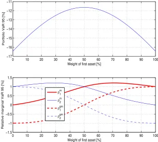
We consider a synthetic portfolio of two uncorrelated assets with zero mean returns and ten percent annual volatility each. Figure 1 displays the results of the sensitivity analysis. The upper part of the figure reports the VaR at the 95% confidence level (VaR95) as a function of the first asset’s weight (in percent) when assuming no leverage in the portfolio (i.e.,w0 = 0). This function is known as thetrade risk profilein the literature. This is the portfolio risk when the portfolio is fully funded. Notice that the VaR95 values are negative percentages since we work with the portfolio return distribution and not with a loss distribution. The portfolio VaR95 is minimized (in the absolute sense) for an equally weighted allocation (VaR95 = -11.63%).

(10)

for this allocation, the portfolio risk is approximately unchanged if we reallocate a small

amount of wealth from the first asset to the second asset (and vice versa). On the other hand, the marginal risk is one percent for both assets, suggesting that leveraging any position will increase (in the absolute sense) the portfolio VaR95.

0 10 20 30 40 50 60 70 80 90 100 −17

−16 −15 −14 −13 −12 −11

Weight of first asset [%]

Portfolio VaR 95 [%]

0 10 20 30 40 50 60 70 80 90 100 −1.5

−1 −0.5 0 0.5 1 1.5

Relative marginal VaR 95 [%]

ρm

1

ρm₂

ρgm

1

[image:10.595.146.455.178.456.2]

ρgm₂

Figure 1: Synthetic portfolio of two assets with equal volatilities and zero correlation. Upper plot: portfolio VaR95 with respect to the first asset’s weight. Lower plot: relative marginal and relative generalized marginal VaR95. Red bold lines: first asset; blue lines: second asset; solid lines: relative marginal VaR95; dashed lines: relative generalized marginal VaR95.

Now, let us assume that the investor has a full allocation in the first asset which corresponds to the very right-hand side of the two plots. In this situation, a moderate levered position in the second asset will have minor impact on the portfolio risk since the marginal VaR95 of the second asset (ρm₂) is zero at this point. On the contrary, the generalized marginal VaR95 (ρgm₂ ) clearly indicates that shifting allocation from the first asset to the second asset decreases the risk in the portfolio.

(11)

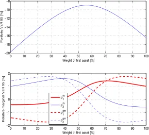
the portfolio VaR95 more than leveraging. Also, note that for a allocation of around 70% in asset one, both sensitivity measures are equal. Reallocation or leverage scenarios lead to the same marginal risk impact in this case.

0 10 20 30 40 50 60 70 80 90 100 −20

−18 −16 −14 −12 −10 −8

Portfolio VaR 95 [%]

0 10 20 30 40 50 60 70 80 90 100 −2

−1 0 1 2

Relative marginal VaR 95 [%]

ρm 1

ρm₂

ρgm 1

[image:11.595.148.456.166.444.2]

ρgm₂

Figure 2: Synthetic portfolio of two assets with unequal volatilities and a negative correlation of -50%. Upper plot: portfolio VaR95 with respect to the first asset’s weight. Lower plot: relative marginal and relative generalized marginal VaR95. red bold lines: first asset; blue lines: second asset; solid lines: relative marginal VaR95; dashed lines: relative generalized marginal VaR95.

4.3. Real-World Portfolio

The generalized marginal risk concept is now examined in a real-world example. We consider a portfolio of equities whose allocations are chosen to replicate the Swiss Market Index (SMI) as of August 27th, 2009. We use monthly closing prices for the SMI constituents ranging from January 2000 to August 2009. Both closing prices and SMI allocation weights are ob-tained from Bloomberg. The monthly arithmetic asset returns are modeled by a multivariate Student-t distribution, where the mean, the covariance matrix and the degrees of freedom parameters are estimated by the EM algorithm.

Figure 3 displays the SMI portfolio weights (left) together with the individual monthly ES at the 95% confidence level (ES95) risk figures. The portfolio is concentrated in half a dozen positions. Individual monthly ES95 range from -12.75% for Nestle to more than -39% for Swiss Life. The overall portfolio ES95 is -12.7%.

(12)

0 5 10 15 20 25 ABB ADECCO ACTELION BAER BALOISE RIECHEMONT CREDIT SUISSE HOLCIM NESTLE NOBEL BIOCARE NOVARTIS ROCHE SWISS RE SWISSCOM SWISS LIFE SYNGENTA SYNTHES UBS SWATCH ZURICH

Portfolio Weights [%]

−40 −30 −20 −10 0

ABB ADECCO ACTELION BAER BALOISE RIECHEMONT CREDIT SUISSE HOLCIM NESTLE NOBEL BIOCARE NOVARTIS ROCHE SWISS RE SWISSCOM SWISS LIFE SYNGENTA SYNTHES UBS SWATCH ZURICH

[image:12.595.146.457.107.332.2]

ES 95 [%]

Figure 3: Left: SMI portfolio weights (in percent). Right: individual monthly ES95.

to decrease the portfolio ES95, the marginal risk suggests to reduce the allocations in ABB first. For instance, reducing the position in ABB by one percent (i.e., from 6.42% to 5.42%) would reduce the portfolio ES95 by 2.15% (i.e., from -12.7% to -12.4%). The component risk analysis indicates that the portfolio risk is concentrated in around half a dozen positions. The hot spots in the portfolio happen to be the holdings with large weights.

0 0.5 1 1.5 2 2.5

Relative marginal ES 95 [%]

0 5 10 15

Relative component ES 95 [%]

Figure 4: Left: (relative) marginal ES95 for the assets in the SMI portfolio. Right: (relative) component ES95.

[image:12.595.147.456.450.677.2]

(13)

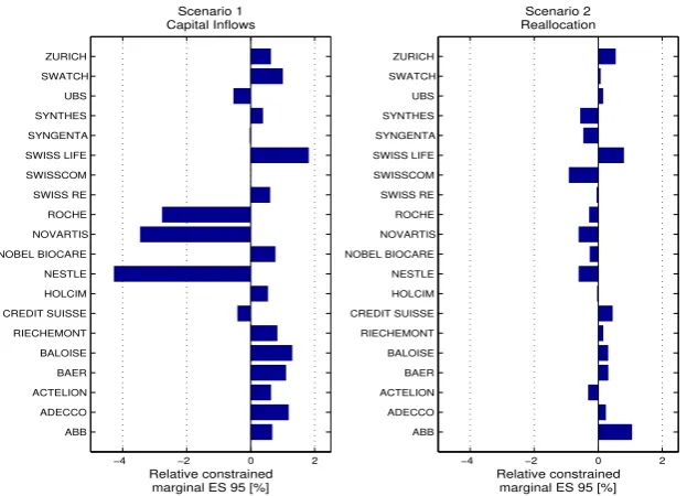
for mutual fund managers and institutional investors which cannot allocate more than a given percentage (often 5%) of the portfolio value on the portfolio cash account. Figure5 displays the results of the sensitivity analysis. The left-hand side reports the generalized marginal ES95 in the case of capital inflows in the portfolio. In this case, additional capital invested in Nestle will have the most effect on decreasing the risk in the new portfolio. For instance, an additional one-percent allocation in Nestle (e.g., from 21% to 22%) would reduce the portfolio risk by 4.27%. On the right-hand side, the case where assets are shifted within the portfolio is displayed. Under this scenario, reallocating capital to Swisscom will decrease the overall risk the most. Note that under the reallocation scenario, the generalized marginal ES95 should be reflective of the return expectations of the portfolio manager. For instance, if the portfolio manager does not have a strong performance expectation on ABB, the position in ABB should be reduced and the proceeds invested equally in the other assets. This sensitivity analysis is especially helpful for an investor who aims at implementing views if a benchmark is to be beaten on a risk-adjusted basis.

−4 −2 0 2 ABB ADECCO ACTELION BAER BALOISE RIECHEMONT CREDIT SUISSE HOLCIM NESTLE NOBEL BIOCARE NOVARTIS ROCHE SWISS RE SWISSCOM SWISS LIFE SYNGENTA SYNTHES UBS SWATCH ZURICH Scenario 1 Capital Inflows Relative constrained marginal ES 95 [%]

[image:13.595.147.459.313.538.2]

−4 −2 0 2 ABB ADECCO ACTELION BAER BALOISE RIECHEMONT CREDIT SUISSE HOLCIM NESTLE NOBEL BIOCARE NOVARTIS ROCHE SWISS RE SWISSCOM SWISS LIFE SYNGENTA SYNTHES UBS SWATCH ZURICH Scenario 2 Reallocation Relative constrained marginal ES 95 [%]

Figure 5: Left: (relative) generalized marginal ES95 for the assets in the SMI portfolio when additional capital is brought in the portfolio and invested in one position (scenario 1). Right: Case where the increase in one position is financed by an equal reduction in all other positions (scenario 2).

5. Conclusion

(14)

proposes a novel approach for measuring the risk sensitivity of a portfolio when the traditional marginal risk fails. The new sensitivity measure, referred to as generalized marginal risk, is based on the directional derivative of the portfolio risk measure. The new metric can deal with cases where the changes in the portfolio results in changes of other position as well. We illustrate the usefulness of the new approach with a synthetic and real-world portfolios within the elliptical framework.

Acknowledgments

The authors wish to thank K. Boudt, C. Davis, K. Deneen, W. G. Hallerbach, L. F. Hooger-heide, C. Ord´as Criado, N. Mirjolet, I. Popovic and O. St¨onner for numerous helpful sug-gestions for improvement of the paper. Finally, the authors thank participants of the 3rd International Workshop on Computational and Financial Econometrics, Limassol, Cyprus.

Disclaimer

The views expressed in this paper are the sole responsibility of the authors and do not nec-essarily reflect those of aeris CAPITAL AG or any of its affiliates. Any remaining errors or shortcomings are the authors’ responsibility.

References

Dowd K (1998). “VaR by Increments.” Risk, pp. 31–32. Special Report on Enterprise-Wide Risk Management.

Duffie D, Pan J (1997). “An Overview of Value at Risk.” Journal of Derivatives,4_{, 7–49.}

Garman M (1996). “Improving on VaR.”Risk,9_{(5), 61–63.}

Garman M (1997). “Taking VaR to Pieces.”Risk,10_{(10), 70–71.}

Gourieroux C, Jasiak J (2009). “Value at Risk.” In Y Ait-Sahalia, L Hansen (eds.), “Handbook of Financial Econometrics,” volume 1, chapter 10. Elsevier Science Ltd.

Gourieroux C, Laurent JP, Scaillet O (2000). “Sensitivity Analysis of Values at Risk.”Journal of Empirical Finance,7_{(3–4), 225–245.} _{doi:10.1016/S0927-5398(00)00011-6}_.

Hallerbach WG (2003). “Decomposing Portfolio Value-at-Risk: A General Analysis.” The Journal of Risk,5_{(2), 1–18.}

Jorion P (2001). Value at Risk: The Benchmark for Controlling Market Risk. McGraw-Hill, Chicago, second edition. (First edition, 1997).

Landsman ZM, Valdez EA (2003). “Tail Conditional Expectations for Elliptical Distributions.”

North American Actuarial Journal,7_{(4), 55–71.}

(15)

Litterman R (1996b). “Hot Spots and Hedges.” Goldman Sachs Risk Management Series.

Litterman R (1997a). “Hot Spots and Hedges (I).”Risk,10_{(3), 42–45.}

Litterman R (1997b). “Hot Spots and Hedges (II).” Risk,10_{(5), 38–42.}

McNeil AJ, Frey R, Embrechts P (2005). Quantitative Risk Management: Concepts, Tech-niques, and Tools. Finance. Princeton University Press, Princeton, USA, first edition. ISBN 0691122555.

Sharpe W (2002). “Budgeting and Monitoring Pension Fund Risk.”Financial Analysts Jour-nal,5_{(5), 74–86.}