An Accurate Five Off Step Points Implicit Block Method for Direct Solution of Fourth Order Differential Equations

(1)

How to cite this paper: Duromola, M.K. (2016) An Accurate Five Off-Step Points Implicit Block Method for Direct Solution of Fourth Order Differential Equations. Open Access Library Journal, 3: e2667. http://dx.doi.org/10.4236/oalib.1102667

An Accurate Five Off-Step Points Implicit

Block Method for Direct Solution of Fourth

Order Differential Equations

Monday Kolawole Duromola

Department of Mathematical Sciences, Federal University of Technology, Akure, Nigeria

Received 12 May 2016; accepted 19 June 2016; published 23 June 2016

This work is licensed under the Creative Commons Attribution International License (CC BY). http://creativecommons.org/licenses/by/4.0/

Abstract

In this article, my focus is the derivation, analysis and implementation of a new modified one-step implicit hybrid block method with five off-step points. The derived method is to solve directly ini-tial value problems of fourth order ordinary differenini-tial equations. The approach for the deriva-tion of the method is to interpolate the approximate power series soluderiva-tion to the problem and to collocate its fourth derivative at the grid and off-grid points to generate systems of linear equa-tions for the determination of the unknown parameters. The derived method is tested for consis-tency, zero stability, convergence and absolute stability. Accuracy and usability of the method are determined with some test problems and the results obtained are found to be better in accuracy than some existing methods.

Keywords

Interpolation, Continuous Coefficients, Block Method, Numerical Integration, Fourth Order Ordinary Differential Equations

Subject Areas: Ordinary Differential Equation

1. Introduction

In sciences and engineering, mathematical models are developed to understand as well as to interpret physical phenomena, many of such phenomena, when modeled, often result into higher order ordinary differential equa-tions of the form:

( )

₍

₎

_{( )}

1 2 3 4

, , , , , , , ,

iv

(2)

OALibJ | DOI:10.4236/oalib.1102667 2 June 2016 | Volume 3 | e2667

equation of the form:

(

,

) ( )

, 0,

[ ]

, , ,

y′ = f x y y a =η f ∈C a b x y∈ℜ (2) and to solve the resulting system of equations by any of the existing methods of solving first order ordinary dif-ferential equations. Literatures abounded in this old conventional method of solving problems of type (1) nu-merically are [1]-[3]. The drawbacks of this method include computational cumbersomeness and longer com-puter tine and space. In addition, [4] observes that these methods do not utilize additional information associated with a specific ordinary differential equation, such as oscillatory nature of the solution. To circumvent these drawbacks, many researchers have solved (1) directly; amongst these are [5]-[7] who develop blocked methods for numerical solution of fourth order ordinary differential equations. [8] develops linear multistep method for solution of fourth order ordinary differential equations whose implementation is Predictor-Corrector mode. Consequently, my motivation in this work is the success story of the adoption of single step method with five off-step points for direct numerical solution of fourth order ordinary differential equations which eliminate the use of predictors by providing sufficiently accurate simultaneous difference equations from a single continuous formula and its derivatives.

2. Derivation of the Method

We take our basis function to be a power series of the form:

( )

( )1

( )

0

r s j j j

y x aψ x

+ −

=

∑

(3)

The fourth derivative of (3) gives

( )

_{( )}

( )1

₍

₎₍

₎

4

_{( )}

0

1 2 3

r s

iv j

j j

y x j j j j aψ x

+ −

−

=

∑

− − − (4)

By putting (4) into (1) we have the differential system:

(

)(

)

( )

(

)

1

4 0

1 2 3 , , , ,

r s

j j j

j j j j a x f x y y y y

+ −

−

=

′ ′′ ′′′

− − − Ψ =

∑

(5)

where a_j’s are the parameters to be determining while r+s denotes number of collation and interpolation

points. By collocating (5) at the mesh points , 0 1

6 n j

x=x₊ j=   

  and interpolating (3) at

1 1 2 5

, , , ,

3 2 3 6

n j

x=x+ j=

yields a system of equations:

(

)(

)

(

)

( )1

4 4

1 2 3 , , , 1, 2, ,

r s

j j n r n r i

j

j j j j aψ x f r o v k i m

+ −

− + +

=

− − − = = =

∑

 (6)

(

)

( )1

0

, , , 0,1, 2, ,

r s

j j n s n s i

j

aψ x y s o v k i m

+ −

+ +

=

= = =

∑

 (7)

By putting these system of equations in the matrix form and then solved to obtain values of parameters aj’s,

1 0, ,

6

j=  which when substituted in (3), yields, after some manipulation, a hybrid linear method with

conti-nuous coefficients of the form:

( )

1

( )

1

( )

4

0 0

j n j j n j

j j

y t α t y+ t h β t f + t

= =

=

∑

+

∑

(8)

The coefficient of αj

( )

t and βj

( )

t are

( )

(

3 2

)

0

1

2 5

8

t t t t

α = + + ,

( )

(

3 2

)

1 3

1

8 22 10

4

t t t t

α = − + + ,

( )

(

3 2

)

1 2

1

10 24 6

2

t t t t

(3)

( )

(

3 2

)

2 3

1

32 18 7 3

4

t t t t

α = − + + + ,

( )

(

3 2

)

5 6

1

3 4

2

t t t t

α = + +

( )

(

8 7 6 5 4 3

)

0

1

12 4 2 4 4 6

19595520

t t t t t t t t

β = + − + − + + −

( )

(

8 7 6 5 4 3

)

1 6

1

258 496 315 998 945 190 178

19595520

t t t t t t t t

β = + − + + − +

( )

(

8 7 6 5 4 3

)

1 3

1

870 9236 7812 7924 7938 7157 5404 836

19595520

t t t t t t t t

β = + − + + + − +

( )

(

8 7 6 5 4 3

)

1 2

1

1840 12846 14410 10450 14224 7102 13368 2784

19595520

t t t t t t t t

β = + + − + − + +

( )

(

8 7 6 5 4 3

)

2 3

1

746 3876 2860 2656 4624 3102 3708 714

19595520

t t t t t t t t

β = + + − + − + +

( )

(

8 7 6 5 4 3

)

5 6

1

22 96 40 136 64 74 88 14

19595520

t t t t t t t t

β = − + − − + − +

( )

(

8 7 6 5 4 3

)

1

5 12 10 8 6 8 14 10

19595520

t t t t t t t t

β = + − + − − + + (9)

where _t x xn vi h

+

−

= .

We evaluate (9) at 0, ,11 6

t= to obtain the discrete one step formula

1 1 2 5

3 2 3 6

4

1 1 1 2 5 1

6 3 2 3 6

10 20 15 4

4 2370 20745 41920 10770 234 25

19595520 n

n n n n

n n

n n n n n

y y y y y

h

f f f f f f f

+ + + +

+

+ + + + +

− + − +

 

= _ + + + + − + _

 

 

(10a)

1 1 1 2 5

6 3 2 3 6

4

1 1 1 2 5 1

6 3 2 3 6

4 6 4

5 51 2679 9854 2679 51 5

19595520

n n n n n

n n

n n n n n

y y y y y

h

f f f f f f f

+ + + + +

+

+ + + + +

− + − +

 

=  − + + + − + 

 

 

(10b)

1 5 2 1 1

6 3 2 3

4

1 1 1 2 5 1

6 3 2 3 6

4 6 4

5 30 54 2504 10029 2574 16

19595520

n

n n n n

n n

n n n n n

y y y y y

h

f f f f f f f

+ ₊ ₊ ₊ ₊

+

+ + + + +

− + − +

 

= _ − + + + + − _

 

 

(10c)

The first derivative of α

( )

t and β

( )

t in (9) gives:

( )

(

2

)

0

1

6 2 5

8

t t t

α′ = + +

( )

(

2

)

1 3

1

24 44 10

4

t t t

α′ = − + +

( )

(

2

)

1 2

1

30 48 6

2

t t t

α′ = + +

( )

(

2

)

2 3

1

96 36 7

4

t t t

α′ = − + +

( )

(

2

)

5 6

1

9 8 1

2

t t t

α′ = + +

( )

(

7 6 5 4 3 2

)

1 6

1

2064 3472 1890 4990 3780 570 178

19595520

t t t t t t t

(4)

( )

(

7 6 5 4 3 2

)

1 3

1

6960 64652 46872 39620 31752 21471 5404

19595520

t t t t t t t

β ′ = + − + + + −

( )

(

7 6 5 4 3 2

)

1 2

1

14880 12922 86460 52250 56896 21306 13368

19595520

t t t t t t t

β ′ = + + − + − +

( )

(

7 6 5 4 3 2

)

2 3

1

5968 27132 17160 13280 18496 9306 3708

19595520

t t t t t t t

β ′ = + + − + − +

( )

(

7 6 5 4 3 2

)

5 6

1

176 672 240 680 256 222 88

19595520

t t t t t t t

β′ = − + − − + −

( )

(

7 6 5 4 3 2

)

1

40 84 60 40 24 24 14

19595520

t t t t t t t

β′ = + − + − − + (11)

Similarly, the second derivative of α

( )

t and β

( )

t in (9) gives

( )

(

)

0

1

12 2

8

t t

α′′ = + 1

( )

(

)

3

1

48 44

4

t t

α′′ = − +

( )

(

)

1 2

1

60 48

2

t t

α′′ = + ₂

( )

(

)

3

1

192 36

4

t t

α′′ = − +

( )

(

)

5 6

1

18 8

2

t t

α′′ = +

( )

(

6 5 4 3 2

)

0

1

672 42 120 40 48

19595520

t t t t t t t

β′ = + − + − +

( )

(

6 5 4 3 2

)

1 6

1

14448 20832 9450 19960 11340 1140

19595520

t t t t t t t

β ′ = + − + + −

( )

(

6 5 4 3 2

)

1 3

1

48720 387912 234360 158480 95256 42942

19595520

t t t t t t t

β′ = + − + + +

( )

(

6 5 4 3 2

)

1 2

1

104160 77532 432300 209000 170688 42612

19595520

t t t t t t t

β′ = + + − + −

( )

(

6 5 4 3 2

)

2 3

1

41776 162792 85800 53120 55488 18612

19595520

t t t t t t t

β ′ = + + − + −

( )

(

6 5 4 3 2

)

5 6

1

1232 4032 1200 2720 768 444

19595520

t t t t t t t

β ′ = − + − − +

( )

(

6 5 4 3 2

)

1

280 516 300 160 72 48

19595520

t t t t t t t

β′ = + − + − + (12)

The third derivative of α

( )

t and β

( )

t in (9) gives

( )

0

1 12 8

t

α′′′ = 1

( )

3

1 48 4

t α′′′ = −

( )

1 2

1 60 2

t α′′′ =

( )

2 3

1 192 4

(5)

( )

5 6

1 18 2

t α′′′ =

( )

(

5 4 3 2

)

0

1

4032 210 480 120 48 1

19595520

t t t t t t

β′′′ = + − + − +

( )

(

5 4 3 2

)

1 6

1

86688 104160 37800 59880 22680 1140

19595520

t t t t t t

β ′′′ = + − + + −

( )

(

5 4 3 2

)

1 3

1

292320 1939560 937440 475440 190512 42942

19595520

t t t t t t

β′′′ = + − + + +

( )

(

5 4 3 2

)

1 2

1

624960 387660 1729200 672000 341376 42612

19595520

t t t t t t

β ′′′ = + + − + −

( )

(

5 4 3 2

)

2 3

1

250656 813960 343200 159360 110976 18612

19595520

t t t t t t

β ′′′ = + + − + −

( )

(

5 4 3 2

)

5 6

1

7392 20160 4800 8160 1536 444

19595520

t t t t t t

β ′′′ = − + − − +

( )

(

5 4 3 2

)

1

1400 2580 1200 480 144 48

19595520

t t t t t t

β′′′ = + − + − + (13)

It is noted that the general fourth order odes involve the first, second and third derivatives. The derivatives can be obtained by imposing that:

( )

1

( )

3

( )

0 0

1 1

i i i i

i i

k k

j n j v n v j n j v n v

j v j v

y x t y t y h t f t f

h α h α β β

−

+ + + +

= =

 

′ = + +  ′ + ′ 

 

∑

(14)

By using (14)and evaluating (11), (12) and (13) at , 0 1 1,

6 n j

x=x₊ j=   

  we obtain the first, second and the

third derivative scheme as follows:

1 1 2 5

3 2 3 6

4

1 1 1 2 5 1

6 3 2 3 6

47 114 93 26

7658 435930 1848915 2845040 696540 14418 1535

195955200 n

n n n n

n n

n n n n n

hy y y y y h

f f f f f f f

+ + + +

+

+ + + + +

′ + − + −

 

−

=  + + + + − + 

 

 

1 1 1 2 5

6 3 2 3 6

4

1 1 1 2 5 1

6 3 2 3 6

26 57 42 11

235 4713 454125 1144150 291225 4935 487

195955200

n n n n n

n n

n n n n n

hy y y y y

h

f f f f f f f

+ + + + +

+

+ + + + +

′ + − + −

 

−

=  + + + + − + 

 

 

1 1 1 2 5

3 3 2 3 6

4

1 1 1 2 5 1

6 3 2 3 6

11 18 9 2

7 14 1000 17960 6445 238 26

195955200

n n n n n

n n

n n n n n

hy y y y y

h

f f f f f f f

+ + + + +

+

+ + + + +

′ + − + −

 

= _ − − − − + − _

 

 

1 1 1 2 5

2 3 2 3 6

4

1 1 1 2 5 1

6 3 2 3 6

2 3 6

134 1101 3960 49270 30750 1611 184

195955200

n n n n n

n n

n n n n n

hy y y y y h

f f f f f f f

+ + + + +

+

+ + + + +

′ + + − +

 

−

=  − + − − + − 

 

(6)

2 1 1 2 5

3 3 2 3 6

4

1 1 1 2 5 1

6 3 2 3 6

6 3 2

134 1122 4425 35440 44580 1146 163

195955200

n n n n n

n n

n n n n n

hy y y y y

h

f f f f f f f

+ + + + + + + + + + + ′ − + − −   =  − + − − + −     

5 1 1 2 5

6 3 2 3 6

4

1 1 1 2 5 1

6 3 2 3 6

2 9 18 11

7 75 385 6690 17715 1147 35

195955200

n n n n n

n n

n n n n n

hy y y y y

h

f f f f f f f

+ + + + + + + + + + + ′ + − + −   − = _ − + − − − + _    

1 1 1 2 5

3 2 3 6

4

1 1 2 5 1

6 2 3 6

11 42 57 26

235 1158 283000 1152375 449190 6358

195955200 n

n n n n

n n

n n n n

hy y y y y

h

f f f f f f

+ ₊ ₊ ₊ ₊ + + + + + ′ + − + −   = _ − + + + _     2

1 1 2 5

3 2 3 6

4

1 1 1 2 5 1

6 3 2 3 6

144 396 360 108

19823 322282 575180 728600 140915 2902 502

10886400 n

n n n n

n n

n n n n n

h y y y y y

h

f f f f f f f

+ + + + + + + + + + ′′ − + − +   = _ + + + + + − _     2

1 1 1 2 5

6 3 2 3 6

4

1 1 1 2 5 1

6 3 2 3 6

108 288 252 72

802 25137 308500 442510 109290 2983 348

10886400

n n n n n

n n

n n n n n

h y y y y y

h

f f f f f f f

+ + + + + + + + + + + ′′ − + − +   − =  − − − − + −      2

1 1 1 2 5

3 3 2 3 6

4

1 1 1 2 5 1

6 3 2 3 6

72 180 144 36

148 2038 30285 196160 53530 978 93

10886400

n n n n n

n n

n n n n n

h y y y y y

h

f f f f f f f

+ + + + + + + + + + + ′′ − + − +   = _ − + + + − + _     2

1 1 1 2

2 3 2 3

4

1 1 1 2 5 1

6 3 2 3 6

36 72 36

7 97 1165 23050 1165 97 7

10886400

n n n n

n n

n n n n n

h y y y y

h

f f f f f f f

+ + + + + + + + + + ′′ − + −   − = _ − + + + − + _     2

2 1 2 5

3 2 3 6

4

1 1 1 2 5 1

6 3 2 3 6

36 72 36

7 42 50 920 23295 1018 48

10886400

n n n n

n n

n n n n n

h y y y y

h

f f f f f f f

+ + + + + + + + + + ′′ − + −   − =  − + + + + −      2

5 1 1 2 5

6

6 3 2 3

4

1 1 1 2 5 1

6 3 2 3 6

36 144 180 72

148 943 2130 48350 20134 27177 1002

10886400

n

n n n n

n n

n n n n n

h y y y y y

h

f f f f f f f

+ + + + + + + + + + + ′′ + − + −   = _ − + + + + − _     2

1 1 1 2 5

3 2 3 6

4

1 1 1 2 5 1

6 3 2 3 6

72 252 288 108

802 5962 19825 137360 414440 325342 19523

10886400 n

n n n n

n n

n n n n n

h y y y y y

h

f f f f f f f

(7)

3

1 1 2 5

3 2 3 6

4

1 1 1 2 5 1

6 3 2 3 6

216 648 648 216

36799 176608 55219 156920 10459 9608 1335

725760 n

n n n n

n n

n n n n n

h y y y y y

h

f f f f f f f

+ + + + + + + + + + ′′′+ − + −   − =  + + + − + −     

3

1 1 1 2 5

6 3 2 3 6

4

1 1 1 2 5 1

6 3 2 3 6

216 648 648 216

1375 46384 148141 81912 29963 3016 391

725760

n n n n n

n n

n n n n n

h y y y y y

h

f f f f f f f

+ + + + + + + + + + + ′′′ + − + −   = _ − − − − + − _     3

1 1 1 2 5

3 6

3 3 2

4

1 1 1 2 5 1

6 3 2 3 6

216 648 648 216

351 3872 54163 114424 15365 1160 151

725760

n n

n n n

n n

n n n n n

h y y y y y

h

f f f f f f f

+ + + + + + + + + + + ′′′ + − + −   − =  − + + + + −      3

1 1 1 2 5

2 3 2 3 6

4

1 1 1 2 5 1

6 3 2 3 6

216 648 648 216

191 1648 7475 39416 28907 2056 231

725760

n n n n n

n n

n n n n n

h y y y y y

h

f f f f f f f

+ + + + + + + + + + + ′′′ + − + −   = _ − + + − + − _     3

2 1 1 2 5

3 3 2 3 6

4

1 1 1 2 5 1

6 3 2 3 6

216 648 648 216

191 1568 6067 35592 32731 3464 311

725760

n n n n n

n n

n n n n n

h y y y y y

h

f f f f f f f

+ + + + + + + + + + + ′′′ + − + −   − =  − + − − + −      3

5 1 1 2 5

6 3 2 3 6

4

1 1 1 2 5 1

6 3 2 3 6

216 648 648 216

351 2608 8531 3080 126709 46792 1415

725760

n n n n n

n n

n n n n n

h y y y y y

h

f f f f f f f

+ + + + + + + + + + + ′′′ + − + −   =  − + − + + −      3

1 1 1 2 5

3 2 3 6

4

1 1 1 2 5 1

6 3 2 3 6

216 648 648 216

1375 10016 31891 78088 33787 177016 36759

725760

n

n n n n

n n

n n n n n

h y y y y y

h

f f f f f f f

+ ₊ ₊ ₊ ₊ + + + + + + ′′′ + − + −   − = _ − + − − − − _     (15)

By combining the schemes (10), the first, second, third derivatives schemes (15) together and write them in block form, using the definition of implicit block method in [9] to obtain the block formula describe as follows:

, , , ,

0 0 1 1

, 0,1, ,

q q q q

p p

i j n j i j n i j n i j n j

j j j j

h a yλ₊ hλ e yλ h −λ d f b f₊ i q

= = + =

 

= + _ + _ =

 

∑

 (16)

λ is the power of the derivative of the continuous method and p is the order of the problem to solved:

q= +r s.

This equation is solved and we obtained values for , ₁, , ₁, , ₁,

i i i i

n v n n v n n v n n v

y₊ y₊ y′₊ y′₊ y′′₊ y′′₊ y′′′₊ and yn′′′+1 as follows: 4

2 3

1 1

6 6

1 1 2 5 1

3 2 3 6

1 1 1

95929 112028

6 72 1296 4702924800

115165 97320 53465 16876 2323

n n n n n

n n

n

n n n n

h

y y hy h y h y f f

f f f f f

(8)

4

2 3

1 1

3 6

1 1 2 5 1

3 2 3 6

1 1 1

4127 8782

3 18 162 18370800

6965 5820 3175 998 137

n n n n n

n n

n

n n n n

h

f f f f f

+ + + + + + +  ′ ′′ ′′′ = + + + +  +   − + − + − _  4 2 3 1 1 2 6

1 1 2 5 1

3 2 3 6

1 1 1

5471 15228

2 8 48 6451200

8775 8120 4455 14040 193

n n n n n

n n

n

n n n n

h

f f f f f

+ + + + + + +  ′ ′′ ′′′ = + + + +  +   − + − + − _  4 2 3 2 1 3 6

1 1 2 5 1

3 2 3 6

2 2 4

1220 3904

3 9 81 1148175

1580 1920 1015 320 44

n n n n n

n n

n

n n n n

h

f f f f f

+ + + + + + +  ′ ′′ ′′′ = + + + + _ +   − + − + −   4 2 3 5 1 6 6

1 1 2 5 1

3 2 3 6

5 25 125

807125 2807500

6 72 1296 188116992

790625 1425000 653125 214256 29375

n n n n n

n n

n

n n n n

h

f f f f f

+ + + + + + +  ′ ′′ ′′′ = + + + + _ +   − + − + −   4 2 3 1 1 6

1 1 2 5 1

3 2 3 6

1 1

191 702

2 6 25200

135 380 135 54 7

n n n n n n

n

n n n n

h

f f f f f

+ ₊ + + + + +  ′ ′′ ′′′ = + + + + _ +   − + − + −   (17) 3 2 3

1 1 1

6 6 3

1 2 5 1

2 3 6

1 1

11458543529 1688294016 16488356235

6 72 26123963443200

13670222640 7552518045 2378490756 326924161

n n n n

n n n

n

n n n

h

y hy h y h y f f f

f f f f

+ + + + + + +  ′ = ′+ ′′+ ′′′+ _ + −   + + + −   3 2 3 1 1 3 6

1 1 2 5 1

3 2 3 6

1 1

13774 35976

3 18 6123600

24465 20800 11370 3576 491

n n n n

n n

n

n n n n

h

y hy h y h y f f

f f f f f

+ + + + + + +  ′ = ′+ ′′+ ′′′+  +   − + − + −   3 2 3 1 1 2 6

1 1 2 5 1

3 2 3 6

1 1

5877 19188

2 8 1075200

8055 8960 4905 1548 213

n n n n

n n

n

n n n n

h

f f f f f

+ + + + + + +  ′ = ′+ ′′+ ′′′+ _ +   − + − + −   3 2 3 2 1 3 6

1 1 2 5 1

3 2 3 6

2 2

3863 13992

3 9 382725

3390 6800 3255 1032 142

n n n n

n n

n

n n n n

h

f f f f f

(9)

3

2 3

5 1 1

6

6 3

1 2 5 1

2 3 6

5 25

505625 1945500 256875

6 72 31352832

1070000 358125 136500 18625

n n n n

n _n _n

n

n n n

h

y hy h y h y f f f

f f f f

+ ₊ ₊ + + + +  ′ = ′+ ′′+ ′′′+  + −   + − + − _  3 2 3

1 1 1 1 2 5 1

6 3 2 3 6

1

198 792 45 480 90 72 7

2 8400

n n n n n n

n n n n n

h

y₊ hy h y h y f f f f f f f ₊

+ + + + +

 

′ = ′+ ′′+ ′′′+  + − + − + − 

 

  (18)

2 3

1 6

2

1 1 1 2 5 1

6 3 2 3 6

1 6

28549 57750 51453 42484 23109 7254 995

4354560

n n

n

n n

n n n n n

y h y h y

h

f f f f f f f

+ + + + + + + ′′ = ′′+ ′′′   + _ + − + − + − _   2 2 3

1 1 1 1 2 5 1

3 6 3 2 3 6

1

1027 3492 1680 1576 873 276 38

3 68040

n n n n

n n n n n n

h

y h y h y f f f f f f f ₊

+ + + + + +   ′′ = ′′+ ′′′+ _ + − + − + − _     2 2 3

1 1 1 1 2 5 1

2 6 3 2 3 6

1

1265 4950 801 2100 1089 342 47

2 53760

n n n n

n n n n n n

h

+ + + + + +   ′′ = ′′+ ′′′+  + − + − + −      2 2 3

2 1 1 1 2 5 1

3 6 3 2 3 6

2

272 1128 18 656 210 72 10

3 8505

n n n n

n n n n n n

h

+ + + + + +   ′′ = ′′+ ′′′+  + − + − + −      2 2 3

5 1 1 1 2 5 1

6 6 3 2 3 6

5

1409 6030 375 4100 225 462 55

6 870912

n n n n

n n n n n n

h

+ + + + + +   ′′ = ′′+ ′′′+ _ + − + − + − _     2 2 3

1 1 1 1 2 5

6 3 2 3 6

41 180 18 136 9 36

840

n n n n

n n n n n

h

y₊ h y h y f f f f f f

+ + + + +

 

′′ = ′′+ ′′′+ _ + + + + + _

 

  (19)

3

1 1 1 1 2 5 1

6 6 3 2 3 6

19087 65112 46461 37504 20211 6312 863

362880

n n n

n n n n n n

h

y h y f f f f f f f ₊

+ + + + + +   ′′′ = ′′′+ _ + − + − + − _     3

1 1 1 1 2 5 1

3 6 3 2 3 6

1139 5640 33 1328 807 264 37

22680

n n n

n n n n n n

h

+ + + + + +   ′′′ = ′′′+  + + + − + −      3

1 1 1 1 2 5 1

2 6 3 2 3 6

685 3240 561 2176 729 216 29

13440

n n n

n n n n n n

h

y h y f f f f f f f₊

+ + + + + +   ′′′ = ′′′+ _ + + + − + − _     3

2 1 1 1 2 5 1

3 6 3 2 3 6

2288 11136 3072 7583 1392 384 64

45360

n n n

n n n n n n

h

y h y f f f f f f f₊

+ + + + + +   ′′′ = ′′′+  + + + + + −      3

5 1 1 1 2 5 1

6 6 3 2 3 6

3715 17400 6375 15384 11625 5640 275

72576

n n n

n n n n n n

h

+ + + + + +   ′′′ = ′′′+  + + + + + −      3

1 1 1 1 2 5 1

6 3 2 3 6

41 216 27 272 27 216 41

840

n n n n

n n n n n

h

y₊ h y f f f f f f f ₊

+ + + + +

 

′′′ = ′′′+ _ + + + + + + _

 

  (20)

3. Analysis of the Properties of the Block

(10)

3.1. Order of the Method

3.1.1. Order of the Block (17)

The linear operator of the block (17) is defined as:

( )

{

:

}

m m

( )

m

( )

m

L y x h =Y −ey +hµ λ− df y +hµ λ− bF y (21)

By expanding y x

(

n+ih

)

and f x

(

n+ jh

)

in Taylor series, (21) becomes:

( )

{

}

( )

2

( )

0 1 2

: p p p

L y x h =C y x +C hy x′ +C h y′′ x ++C h y x (22)

The block (17) and associated linear operator are said to have order p if

0 1 p3 0, p 4 0.

C =C ==C ₊ = C ₊ ≠ See [10].

The term Cp+4 is called the error constant and implies that the local truncation error is given by:

( 4) ( 4)

_{( )}

( 5)

4 0

p p p

n k p n

t+ =C + h + y + x + h + (23)

Hence the block (17) has order 7 with error constant:

T

4

15739 733 1

10861273143705600 33941478574080 11496038400

37 198125 1

165729875850 434450925748224 1231718400

p

C +

 

 

=  

 

 

3.1.2. Order and Error Constant of the Main Method (10c)

By rewriting the main method (10c) in the form:

1 5 2 1 1

6 3 2 3

4

1 1 1 2 5 1

6 3 2 3 6

4 6 4

5 30 54 2504 10029 2574 16 0

19595520 n

n n n n

n n

n n n n n

y y y y y

h

f f f f f f f

+ ₊ ₊ ₊ ₊

+

+ + + + +

− + − +

 

− _ − + + + + − _=

 

 

(24)

Expanding (24) in Taylor series in the form:

( ) ( ) ( ) ( ) ( )

( ) ( )

0 0 0 0 0

4 4

0

5 2 1 1

4 6 4

! 6 ! 3 ! 2 ! 3 !

30 1 54 1 2504 1

! 19595520 6 19595520 3 19595520 2

10029 19595520

j j j j

j j j j j

n n n n n

j j j j j

j j j

j j n j

h h h h h

y y y y y

j j j j j

h y j

∞ ∞ ∞ ∞ ∞

= = = = =

+ ∞

+ =

       

− _{ } + _{ } − _{ } + _{ }

       

 ₋ _{ } _{ } _{ }

−   _{ } +  _{ } +  _{ }



+

∑

( )4 4

2 2574 5 16 5

0

3 19595520 6 19595520 19595520

j j

n

h y 

  ₊   ₋ ₋ ₌



   

    _

(25)

Since C0,,C10 =0 but C11≠0 see [10]; then the main scheme is of order 7 and the error constant is:

4

1 1097098297344

p

C + = .

3.2. Zero Stability of the Block

The block (17) is said to be Zero stable if the roots zs=1, 2,,N of the characteristic polynomial

( )

z det

(

zA E

)

ρ = − , satisfies z ≤1 and the root z =1 has multiplicity not exceeding the order of the diffe-rential equation. Moreover as

( )

(

)

0, r 1

hµ → ρ z =z−µ λ− ,

(11)

( )

5

(

)

1 0 0, 0, 0, 0, 0,1

z

ρ =λ λ− = ⇒ =λ

Hence our method is Zero stable.

3.3. Consistency of the Main Method (10c)

From main method (10c), the first and second characteristics polynomials of the method are given by:

( )

_r _r ₄_r65 ₆_r32 ₄_r12 _r31

ρ = − + − +

and

( )

16 23 12

1 5

3 6

5 30 54 2504

19595520 19595520 19595520 19595520

10029 2574 16

19595520 19595520 19595520

r r r r

r r r

σ = − + +

+ + −

the method (10c) is consistent since it satisfies the following conditions: 1. The order of the method is p= ≥7 1 which is obvious.

2. For the method α =1 1, 5 6

4

α = − , 2 3

6

α = , 1 2

4

α = − and 1

3

1

α = , thus

1 1

1 4 6 4 1 0, 1

3 6

j j

j

α = − + − + = _{=  }   

∑

.

3.

( )

5 2 1 1

6 3 2 3

4 6 4

r r r r r r

ρ = − + − + .

4. it follows from here that ρ

( )

1 = =0 ρ′

( )

1 showing that the condition (3) is satisfied as well. 5. Note that:

( )

_{( )}

455 136 112 103 15 72 80 113

324 27 4 81

iv

r r r r r

ρ = − − − + − − −

( )

_{( )}

1 4! 1

iv

ρ σ

⇒ = .

For the principal root r = 1: it is observed that the last condition above is satisfied, hence the main method is consistent.

3.4. Convergence

The necessary and sufficient condition for a numerical method to be convergent is for it to be consistent and Zero stable. Thus since it has been successfully shown from the above condition, it could be seen that our me-thod is convergent.

3.5. Region of Absolute Stability of the Method We consider the stability polynomial written in general form:

( )

r h,

( )

r h

( )

r 0

π =ρ − σ =

where h=h2λ and df

y λ

δ

= is assumed constant. The stability polynomial of the main method (10c)

be-comes:

5 2 1 1 1 1

0

6 3 2 3 6 3

2 5

1

3 6

2

5 30 54

4 6 4

19595520 19595520 19595520

2504 10029 2574 16

0

19595520 19595520 19595520 19595520

r r r r r h r r r

r r r r

  

− + − + − − +

  

  



+ + + − _=



(12)

Adopting the boundary locus method whose equation is given by:

( )

r h

r ρ σ

= (27)

By inserting the values of ρ

( )

r and σ

( )

r into (27) and evaluate, we obtain the following results as dis-played in the table below:

θ 0 30 60 90 120 150 180

( )

h θ 0 −0.075 −1.203 −6.088 −19.241 −46.976 −96.407

From here, it could be seen that the region of absolute stability of the method is given by x

( ) (

θ = −96.407, 0

)

which satisfies the condition for A-stability, similarly the interval of periodicity lies in interval x

( ) (

θ = −∞, 0

)

.

4. Numerical Experiments

To test the accuracy, workability and suitability of the method, I adopted our method to solving some initial value problems of fourth order ordinary differential equations.

Test Problem 1

I consider special fourth order problem:

( )

0 0,

( )

0 1,

( )

0 0,

( )

0 0, 0.1 iv

y x

y y y y h

=

′ ′′ ′′′

= = = = =

Whose exact solution is:

( )

5

120

x

y x = +x

My method was used to solve the problem and result compared with [6]. The result is as shown inTable 1.

Test Problem 2

I consider a linear fourth order problem

π 0, 0

2

iv

y +y′′= ≤ ≤x

( )

1.1

( )

1 1.2 0.1

0 0, 0 , 0 , ,

72 50π 144 100π 144 100π 32

y = y′ = y′′ = y′′′= h=

− − −

Whose exact solution is given by:

( )

1 cos 1.2 sin

144 100π

x x x

y x = − − −

−

My method was used to solve the problem and result compared with [8]. The result is as shown inTable 2.

Numerical Results

I make use of the following Notations in the table of results:

XVAL: Value of the independent variable where numerical value is taken. ERC: Exact result at XVAL.

NRC: Our Numerical result at XVAL. ERR: Error of our result at XVAL.

5. Discussion of Results

(13)

[image:13.595.86.538.99.295.2]

OALibJ | DOI:10.4236/oalib.1102667 13 June 2016 | Volume 3 | e2667 Table 1.Showing results for problem 1.

XVAL ERC NRC ERR P = 7 K = 1 ERR in [6] P = 4 K = 6

0.1 0.1000000833333340 0.10000008333349980 1.658E−13 7.000E−10

0.2 0.20000266666666690 0.20000266666998294 3.316E−12 8.999E−10

0.3 0.300020250000000004 0.30002025000718312 7.183E−12 2.999E−09

0.4 0.400008533333333333 0.40000853339982528 6.649E−11 5.100E−09

0.5 0.500260416666666665 0.50026041667657280 9.906E−11 7.799E−09

0.6 0.600648000000000007 0.60064800003216824 3.217E−11 1.180E−08

0.7 0.701400583333333344 0.70140058343576487 2.432E−10 1.240E−08

0.8 0.802730666666666670 0.80273066698686870 3.202E−10 1.410E−08

0.9 0.904920750000000005 0.90492075025408587 2.540E−10 1.880E−08

[image:13.595.88.536.317.504.2]

1.0 1.00833333333333300 1.00833333359573400 2.024E−10 2.600E−08

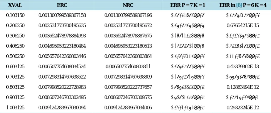
Table 2. Showing results for problem 2.

XVAL ERC NRC ERR P = 7 K = 1 ERR in [8] P = 6 K = 4

0.103150 0.001300799589367158 0.001300799589367196 0.38142683E−18 0.49873299E−15

0.206250 0.002531773700195635 0.002531773700195672 0.37184370E−17 0.67654215E 15

0.306250 0.003652478978884993 0.003652478978887675 0.26822346E−16 0.31350790E−14

0.406250 0.004695953223180484 0.004695953223180513 0.29384802E−16 0.94360283E−13

0.506250 0.005657642360803446 0.005657642360803864 0.41813224E−15 0.22116856E−13

0.603125 0.006507754608034524 0.00650775460803811 0.38734880E−15 0.43379362E 13

0.703125 0.007298314767638522 0.007298314767638809 0.28714827E−15 0.77870869E−13

0.803125 0.007998520222728983 0.007998520222737657 0.86740034E−14 0.12863494E 12

0.903125 0.008607246703302495 0.008607246703309575 0.70802448E−14 0.19927115E−12

1.003125 0.009124283967030094 0.009124283967034006 0.35121472E−14 0.29323245E 12

The order of my method is of order 7 higher than that of [6] of order 4, which collaborates the principle, that the higher the order of a method is, the more accurate it is. The absolute errors in [6] are more than those of the new methods; this also means that the new methods are accurate than [6] which is of order 4 and implemented in block mode.

The results of my new method when also compared with the block method proposed by [8] showed that my method is more accurate.

References

[1] Lambert, J.D. (1973) Computational Methods in ODEs. John Wiley & Sons, New York.

[2] Fatunla, S.O (1991) Block Method for Second Order IVPs. International Journal of Computer Mathematics, 41, 55-63.

http://dx.doi.org/10.1080/00207169108804026

[3] Brujnano, L. and Trigiante, D. (1998) Solving Differential Problems by Multistep Initial and Boundary Value Methods. Amsterdam, Gordon and Breach Science Publishers, Netherlands.

[4] Vigo-Aguiar, J. and Ramos, H. (2006) Variable Step Size Implementation of Multistep Method for y′′= f x y y

(

, , ′

)

.

Journal of Computational and Applied Mathematics, 192, 114-131.http://dx.doi.org/10.1016/j.cam.2005.04.043

(14)

Putra, Malaysia.

[6] Mohammed, U. (2010) A Six Step Block Method for Solution of Fourth Order Ordinary Differential Equations. The Pacific Journal of Science and Technology, 11, 258-265

[7] Ademiluyi, R.A, Duromola, M.K. and Bolaji, B. (2014) Modified Block Method for the Direct Solution of Initial Val-ue Problems of Fourth Order Ordinary Differential Equations. Australian Journal of Basic and Applied Sciences, 8, 389-394.

[8] Kayode, S.J. (2008) A Zero StableMethod for Direct Solution of Fourth Order Ordinary Differential Equation. Ameri-can Journal of Applied Sciences, 5, 1461-1466.http://dx.doi.org/10.3844/ajassp.2008.1461.1466

[9] Shampine, L.F. and Watts, H.A. (1969) Block Implicit One Step Methods. Mathematics of Computation, 23, 731-740.

http://dx.doi.org/10.1090/S0025-5718-1969-0264854-5