http://dx.doi.org/10.4236/ijmnta.2013.24028
Dynamics of a Hyperparasitic System with Prolonged
Diapause for Host
*
Limin Zhang1#, Chaofeng Zhang1,2 1
Department of Mathematics and Finance-Economics, Sichuan University of Arts and Science, Dazhou, China 2
School of International Trade and Economics, University of International Business and Economics, Beijing, China Email: #[email protected], #[email protected]
Received October 9,2013; revised November 9, 2013; accepted November 17, 2013
Copyright © 2013 Limin Zhang, Chaofeng Zhang. This is an open access article distributed under the Creative Commons Attribution License, which permits unrestricted use, distribution, and reproduction in any medium, provided the original work is properly cited.
ABSTRACT
A hyperparasitic system with prolonged diapause for host is investigated. It is assumed that host prolonged diapause occur at larval stage, and parasitoid attack is limited to egg stage before the initiation of host diapause. Such behavior has been reported for many ichneumons. Hyperparasite only attacks the parasitoids that parasitize the hosts. Hyperpara-sitic system is often used in biological control. The existence and stability of nonnegative fixed points are explored. Numerical simulations are carried out to explore the global dynamics of the system, which demonstrate appropriate prolonged diapause rate and appropriate intrinsic growth rate can stabilize the system. The reasons are explained ac-cording to the ecological perspective. Furthermore, many other complexities which include quasi-periodicity, pe-riod-doubling bifurcations leading to chaos, chaotic attractor, intermittent and supertransients are observed.
Keywords: Hyperparasitic System; Prolonged Diapause; Dynamic Complexities
1. Introduction
Hosts and parasitoids are mostly univoltine and have no overlap between successive generations. Therefore, their interactions can be modeled by discrete differences. An early work by Beddington et al. [1] showed that discrete host-parasitoid models can produce a richer set of dy-namic patterns than those observed in continuous-time models. More recently, many researchers [2-12] have reported that discrete host-parasitoid models can have very complex dynamics.
However, few studies have explored hyperparasitic systems using mathematical approaches and difference equations. Actually, hyperparasite can play a crucial role in the control of a host-parasitoid interaction if they are successfully established in the community. Furthermore, few works on complex dynamics in parasitic system have considered diapause. In the natural world, many insects which inhabit unpredictable environments display dia-pause for one year or more, which can be described as prolonged or extra-long diapause [13]. As observed in
numerous laboratory and field experiments, diapause is induced by changing responses to temperature, photope-riod, humidity, hormonal treatment and other factors [14- 16]. Thus, incorporating hyperparasite and diapause in parasitic system is more realistic and more practical sig-nificance.
In the paper, a hyperparasitic system with prolonged diapause for host is investigated. In the system, we as-sume that host prolonged diapause occur at larval stage, and parasitoid attack is limited to egg stage before the initiation of host diapause. The parasitoids are physio-logical “regulators” [17]. In this case, the parasitoid can potentially attack all hosts, but do not undergo prolonged diapause itself. Such behavior has been reported for many ichneumons [18]. Hyperparasite only attacks the parasitoids that parasitize the hosts [19]. Based on the above considerations, the model can be represented by the following difference equation:
1 1
1 1 1
1 1 2
1 1
1 exp 1
exp 1
1 exp exp
1 exp 1 exp
t t t t
t t
t t t t
t t t t
h d h r h k a p
d h r h k a p
p h a p a q
q h a p a q
12 t
, (1)
*This work is supported by the National Natural Science Foundation of
China (No. 30970305), the Sichuan Provincial Natural Science Founda-tion (No. 13ZB0102).
where denote the densities of the host, parasi-toid, hyperparasite respectively at generation . In the absence of parasitism, the host adapts to Moran-Ricker model [20,21], that is to say
, ,
t t t
h p q
t
1 exp 1
t t t
h h r
h k
,
where is the intrinsic growth rate and is the car-rying capacity. The function exp 1 t given by Poisson distribution proposed by Nicholson and Bailey [22] stands for the probability that a host escapes parasit-ism,where 1 is the parasitoid searching efficiency. By analogy with the above, the probability that a parasitoid escapes hyperparasites is
r
a
k
a p
a q2 t
exp . Accordingly, 2 is the hyperparasite searching efficiency. The parameters
and
a
d represent diapause rate and survival rate of the host, respectively. According to their biological meaning, d and are non-negative and less than 1.
2. Stability Analysis
In this section, the existence and asymptotic stability analysis of the non-negative equilibrium points of system (1) are investigated. The system has four non-negative equilibrium points which are given by the following statements:
a) The equilibrium point E1
0, 0, 0
always exists. b) The positive equilibrium point
*
is2 , 0, 0
E h
given by h*k1 ln 1
d d r
which exists if and only if
ln 1 0.
r d d (2) The positive equilibrium point is given
by
3 ˆ ˆ, , 0
E h p
1
1
ˆ 1 ln 1 ˆ ,
ˆ
ˆ 1 exp ˆ ,
h k d d a p r
p h a p
(3) which exists if and only if
1ˆln 1 .
r d d a p
(4) The positive equilibrium point is given
by
4 , ,
E h p q
1
1 2
1 2
1 ln 1 ,
1 exp exp ,
1 exp 1 exp ,
h k d d a p r
p h a p a q
q h a p a q
p
(5)
which exists if and only if
1ln 1 .
r d d a (6) Analysis of the stability of the system (1) close to the above equilibrium points requires that the system is fully specified in terms of densities at time and . For this, we introduce two variables, t and t, corre-sponding to the densities of hosts and parasitoids at time
respectively. Then the system (1) corresponds to the following form:
1
t t
w v
1
t
1 1
1
1 1 2
1 1
1 1
1 exp 1
exp 1
1 exp exp
1 exp 1 exp
, .
t t t t
t t t
t t t t
t t t t
t t t t
h d h r h k a p
d w r w k a v
p h a p a q
q h a p a q
w h v p
2
(7)
Accordingly, the four equilibrium points of the system (1) corresponds to the following forms respectively:
1 2
3 4
0, 0, 0, 0, 0 ,
1 ln 1 , 0, 0,
1 ln 1 , 0 .
ˆ, , 0, ,ˆ ˆ ˆ , , , , , .
E
E k d d r
k d d r
E h p h p E h p q h p
The stabilities of equilibrium points , , 3 and 4 are as the same as these points 1 2 3 and 4 respectively. Now we study the linear stability of fixed points in the system (7). The Jacobian matrix at an arbi-trary
1
E E
2
E E
E
E E E
h p q h p, , , ,
is given by11 12 11 12 21 22 23
31 32 23
0
1 1
0 0
0 0
1 0 0 0 0
0 1 0 0 0
d d
f f f
d d
f f f
J
f f f
f
,
where
11 1
12 1 1
21 1 2
22 1 1 2
23 2 1 2
31 1 2
32 1 1 2
1 1 exp 1
1 exp 1 ,
1 exp exp ,
exp ,
1 exp exp ,
1 exp 1 exp ,
exp 1 exp .
f d rh k r h k a p
f a d h r h k a p
f a p a q
f a h a p a q
f a h a p a q
f a p a q
f a h a p a q
The characteristic equation of J is
4 3 2
3 2 1 0 0
H f f f f , (8) where
2
0 12 11 22
12
1 2
11 22 2 2 22
, 1
1
, 1
a d p q p
f f f f
d h
pf d
f a p q
h d
d
f f a p q a p f
d
2 12 11 22 2 2 22
3 2 22
, 1
1
1 .
1
p d
f f f f a p a f p q
h d
d r
f a p h f
d d k
r
Moreover, an application of the local stability analysis of the system (7), gives the following results:
(1) Substituting the fixed point into the Equation (8), we get
1
E
3 2
e 1r d d e 0
. (9)
The roots of the Equation (9) are 1,2,30,
2
24,5
1 e e 1 4 e
. 2
r r
d d
r
d
The modulus of 1, 2,3 is less than one. Then is local stability if and only if
1
E
2
21 e e 1 4 e
1
2
r r r
d d d
1
1
,
which yields
(10)
1 d d
er (2) Substituting the fixed point into the equation (8), we get
2
E
2 2
22 11 11 0
1
d
a a a
d
, (11)
where
* *
11 22 1
*
1
1 ,
1
ln 1 1
d r
a h
d d k
d d h k
r
a a h .
Several roots of the Equation (11) are 1,2 0, 3 a22
. Obviously, the modulus of 1, 2 is less than one. The modulus of 3 is less than one if and only if
1 ln 1
0.r a k r d d (12) Under the conditions of (2) and (12), the stability of
is identified by the equation
2
E
2
11 11 0
1
d
a a
d
. (13)
It follows from the well-known Schur-cohn criterion [23] that the modulus of all roots of the Equation (13) is less than one if and only if
11 11 11 11
11
1) 1 0, 2)1 0
1 1
3) 1. 1
d d
a a a a
d d
d a d
. (14)
From the inequalities (12) and (14), we obtain the fol-lowing conditions for the stability of 2:
Proposition 1. The equilibrium point 2 is locally
stable if and only if the following conditions hold:
E E
1
0 ln 1
2 1 1
min , , 2
1
r d d
d r d
d d a k d
. (15)
Proof. From the conditions (15), we can know the ine-qualities (2) and (12) obviously hold. Let's study the inequalities (14).
1) 1 11 11 ln 1
1
d
a a r d d
d
0
.
2)
11 11
1
1
2 1 1
ln 1
1 1
d
a a
d
d d d
r d d
d d d d
.
When 1 d d 0, according to the conditions (15), we obtain 1 11 11 0
1
d
a a
d
.
When 1 d d 0, according to the conditions (15), we obtain
11 11
2 1
1 0
1 1
d d
a a
d d d
.
3)
11 ln 1 1
1 1
1
1 1
1
d d
a r d d
d d d
d d
d d d
.
Obviously,
11 ln 1 1
1 1
1 1
d d
a r d d
d d d
d
d d
Therefore, if the conditions (15) are satisfied, the equi-librium point 2 is locally stable.
(3) Substituting the fixed point into the Equation (8), we get
E
3
E
3 2
2ˆ 2 1 0 0
a p
(16)
where
0 1 11 12 1 1 11 12 11 2 1 11
ˆ
ˆ ˆ
ˆ 1
ˆ
ˆ ˆ ,
ˆ 1
ˆ ˆ
d p
a b h p b
d h
p d
a b h p b b
d h
a h p b
11 1
12 1 1
1
ˆ ˆ ˆ
1 1 exp 1
1 ˆ
1 ,
1
ˆ ˆ ˆ
1 exp 1
ˆ
1 1 0,
r r
b d h r h a
k k
d r
h
d d k
b a d h r h k a p
a d h d d
p
Two roots of the Equation (16) are 1 0, 2 a p1ˆ. Obviously, the modulus of 1 is less than one. The modulus of 2 is less than one if and only if
2ˆ 1
a p . (17) Under the conditions of (4) and (17), the stability of
is identified by the equation
3
E
3 2
2 1 0 0
. (18) By analogy with the above, the modulus of all roots of the Equation (18) is less than one if and only if
2 1 0 2 1 0
2
0 0 1 2 0
1 0,1
1 1,1 0.
0, 2 , (19)
are satisfied. Based on the above analysis, we obtain the following sufficient conditions for the stability of 3.
Proposition 2. The equilibrium point is locally
stable if the following conditions hold:
E
3
E
1: ln 1 1ˆ, ˆ 1
H r d d a p a p
2: ˆ ;
k H h r
1 3 1 1 1 ˆ ˆ ˆ: max , 0
ˆ 1
1
ˆ
min 1 ,
ˆ
2 1 1
ˆ .
ˆ
1 2 1
a pk d
H a h p
d k rh
d k
a p
d k rh
d k d d
a p
d d k rh d d
Proof. We only need verify the inequalities (19). Ac-cording to the condition H2, we obtain 11 .
Substitute the signs of 11 and , we get
0
b
b b12 00, 2 0
. Substituting the values of b11, b12 for 1 and rearranging the term we get
1 1 ˆ 1 ˆ ˆ 1d k rh d
a h p a p
d d k d
1ˆ
1
According to the condition H3, we obtain 10. By analogy with 1, we get
0 1
ˆ
ˆ ˆ ˆ 1
1
d k rh
a h p a p
d d k
1
0 .According to the signs of , we obtain 2 1
0,1, 2i i
0
1 . Now, we prove the fourth inequality of (19).
20 1 2 0 2
0 1 2 0 0 1 2 0 1 2
1 11 11 12 1 1 1 1 1 1 1 ˆ ˆ 1 1 1 ˆ 1 1 ˆ 1 1 ˆ ˆ 2 1
ˆ ˆ ˆ
1 .
1
d d
a h p b
d
d d d d p
b b
d d h
k rh d d k rh
a h p a p
k d d k
.
According to the conditions H2 and H3, we obtain
0 1 2
1 0. That is to say 2
0 1 2 0
1 0
0
1 1
. At the same time,
2 1 2 1 0 0
. The proof is com-plete.
(4) Substituting the fixed point into the equation (8), we get
4
E
4 3 2
3 2 1 0 0
c c c c
, (20)
where
20 12 11 22
12
1 2
11 22 2 2 22
2 12 11 22 2 2 22
3 2 22
11 , 1 1 , 1 , 1 1 1 1 1 1
a d p q p
c c c c
d h
pc d
c a p q
d h
d
c c a p q a p c
d
p d
c c c c a p a c p q
d h
d r
c a p h c
d d k
c d rh k
112 1 1
1
22 1 1 2 1
exp 1
1 1 1 ,
1 exp 1
1 1 0,
exp 0 .
r h k a p
d d d rh k
c a d h r h k a p
a h d d d
c a h a p a q a p h p q p q
Under the condition of (6), the stability of is identified by the following equation
4
E
4 3 2
3 2 1 0 0
c c c c
3 2 1 0 3 2 1 0 2
0 0 1 3 0
2 2
2
0 1 3 0 2
0 0 2 1 3 0 3 1 0
1 0,1
1 1,1 0,
1
1 1
c c c c c c c c
c c c c c
c c c c
c c c c c c c c c
0, 0. (22)
are satisfied. Based on the above analysis, we obtain the following sufficient conditions for the stability of 4.
Proposition 3. Under the condition of (6), the equilib-rium point is locally stable if the following condi-tions hold: E 4 E
1 1 2 2 2 3 2 1 2 1 2 4 1 1: , 0 1
: 1 0,
1 1 0, 1 1 1 : 1 1 1 1 1 . 1 1 : 2 1
k r d d
W h B
r k d a a ph
r d
W A h a B D
k d
d
M N
d d
d r d
W h a B
d d k a p d
a hd r
A B D
d k a p
d
W M a p D
d d D 2
1 2 0.
1
r d
A h a B D N
k d where
2 2 1 1 2 1 + ; 1 ; ; + ; . + 1 d A a p qd
a h p q B h p q D
p q a
a ph d
2
M a p N a a pB
p q d
Proof. According to the condition W1, we obtain
11 . Substitute the signs of c11, 12 and , we get , 3 . Substitute the values of , and , we get
0 c 0 c 22 c
c c22
11
c
0
c 0 c12
1 2 0 1 1 2 2 1 , 1 1 1 , 1 1 1 . 1 anda a phd r
c B
d d k
d a p r d
c A h a B
d d k d
d
c M N
d d D
1
3 2 1 0
1 c c c c 0
,
By the conditions and , we obtain , and . Then, it is easy to verify
1
W W2 0c0
1 0
c c20
. And.
2
0 1 3 0 2
0 3 0 1 0 3 1 0 3 1
1
1 2
1 2
1
1 1 .
1 1 1 1 1 1 1 1 . 1
c c c c
c c c c c c c
c c c
d a pD
d d
r r d
h a p A h a B D
k k
a a phd r B d k d
According to the condition W3, we obtain
0 3 1
1 c c c 0. That is to say 2
0 1 3 0
1c c c c 0 0
c
. According to the conclusion 2 , we obtain 1 c3 c2 c1 c00 . Now, we prove the fifth inequality of (22).
20 0 2 1 3 0 3 1 0
0 2 1 3 2 1 3
2 1 3
1 2 1 2 1 2 1 1
1 2 .
1 2 1 2 1 1 1 1 2 1 1 2 1 1 1
c c c c c c c c c
c c c c c c c
d c c c
d d
r d
M a p A h a B D
k d
d r
a pD h N
d d k
d
M a p D
d d
r d
A h a B D
k d
2N 0
.
By the condition W4, we obtain
2 2 20 1 3 0
2
0 0 2 1 3 0 3 1 0
2 2
2 2
0 3 0 1 0 0 2
1 3 0 3 1 0
2 2
0 3 0 1 3 0 1 3 0 1 0 2
3 0 1 3 1 0
3 0 1 0 3 2 1 0
1
1 1
1 1 1
1 1
1 1 0.
c c c c
c c c c c c c c c
c c c c c c c
c c c c c c
c c c c c c c c c c c c
c c c c c c
c c c c c c c c
The proof is complete.
3. Numerical Simulations
on to explore the possibilities of dynamical behaviors for system (1).
3.1. Bifurcation Analysis
In the section, a one-dimensional bifurcation analysis is carried out to investigate the overall dynamic behavior of the system. One-dimensional bifurcation diagrams give information about the dependence of the dynamics on a certain parameter. The analysis is expected to reveal the type of attractor to which the dynamics will ultimately settle down after passing an initial transient phase and within which the trajectory will then remain forever [2]. The bifurcation parameters are considered in the follow-ing two cases:
1) Varying d in the range , and keeping other parameters fixed as below:
0 d 1
0.472
, a10.2, a20.3, r3, k20. (23) 2) Varying in the range , and keeping other parameters fixed as below:
r 2 r 4.3
0.472
, a1 0.2, a20.3, d0.235, k20. (24)
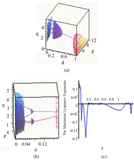
Figure 1(a) shows the bifurcation diagram in the
space with the parameters given by case 1). As increases from to , the system is cha-otic. Subsequently the chaotic attractor abruptly disap-pears and a period-4 attractor apdisap-pears which constitute a type of attractor crisis. In the range , the system passes through a quasi-periodic band with fre-quency-lockings and tangent bifurcations. As further increases, a period-2 attractor appears. When in-creases from to , the system goes through a quasi-periodic band with frequency-locking and tan-gent bifurcation. As is slightly beyond , a sta-ble coexistence of the system is observed. When in-creases beyond , the system crosses a chaotic band. When is slightly increased beyond , the hy-perparasite population is extinct, while the parasitoid population enters another chaotic band with period win-dows. Figure 1(b) is the local amplifications of Figure
1(a) with .
d p q
d
d
0
.18
0.0389
2
0.075, 0.08
d d
0.482
0.9482 0.167
0.86
0 d 0
0.48
d
7
d
The Maximum Lyapunov exponents have been proved to be the most useful dynamic diagnostic tool for chaotic systems. It is the average exponential rate of divergence or convergence of nearby orbits in phase space [24]. The Maximum Lyapunov exponents corresponding to Figure 1(a) are given in Figure 1(c), which are in agreement with the bifurcation diagram. When , the Maximum Lyapunov exponents change from positive to negative, which corresponds with the system changing from chaos to period. In the range , the Lyapunov exponents fluctuate around 0 with very small
0 d 0.07
0.075, 0.08(a)
(b) (c)
Figure 1. (a) Bifurcation diagram in d p q space; (b) The magnified part with 0 d 0.18; (c) The Maximum Lyapunov exponents corresponding to (a). The other pa-rameters are fixed as Equations (23).
amplitude standing for quasi-periodicity, which are the same as in the range
0.167, 0.482
d
. As increases from to , the Maximum Lyapunov expo-nents are negative, corresponding to a stable coexistence of the system. When is slightly increased beyond
, Most of the Maximum Lyapunov exponents are positive and few are negative. So there exist period win-dows in the chaotic band.
d
0.482 0.867
0.867
As can be seen from Figure 1, the behaviors of the system are very complicated, including stable coexis-tence, chaotic bands with period windows, quasi-perio- dicity with frequency-locking. Furthermore, from an ecological point of view, it is apparent that appropriate prolonged diapause rate can moderate coexistence. The reason is that appropriate diapause rate helps the fraction hosts to escape parasitism, but high diapause goes against the parasitoid growth.
4
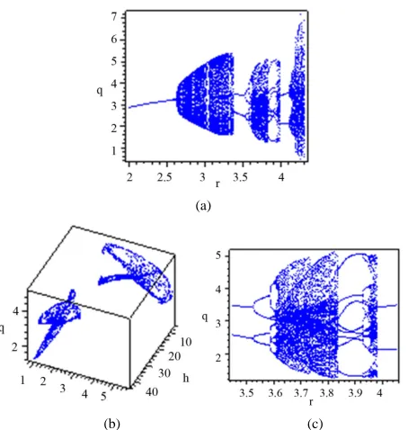
Figure 2(a) shows the bifurcation diagram in the
rq plane with the parameters given by case (Ⅱ). As the parameter increases from to 2.603, a stable coexistence of the system is observed. As further increases, a Hopf bifurcation occurs at
r 2
r
r2.60348. Then the system enters quasi-periodicity, including fre-quency-lockings and tangent bifurcations. When
3.
[image:6.595.312.535.82.348.2](a)
(b) (c)
Figure 2. (a) Bifurcation diagram in plane; (b) The
chaotic attractor at ; (c) The magnified part with
. The other parameters are fixed as
Equa-tions (24).
rq 3.8
r 3.45 r 4.51
the same as in the range
. A typical chaotic attractor is presented in Figure 2(b) at . Subse-quently the chaotic attractor abruptly disappears and a period-2 attractor appears. When increases from 4.145 to 4.5, the system enters a chaotic band again.Figure 2(c) is the local amplifications of Figure 2(a)
with .
3.838, 3.935
r
3.8
r
3.45 r 4.51
From Figure2, we can know that appropriate intrinsic growth rate can stabilize the system, but the high intrinsic growth rate may destabilize the stable dynamics into more complex dynamic. The reason is that the population would increase over carrying capacity with high intrinsic growth rate and then lose its stability.
r
3.2. Intermittent Chaos and Supertransients
Intermittency as illustrated in Figure 3(a) is character-ized by switches between apparently regular and chaotic behaviors even though all the control parameters are constant and no external noise is present [25]. The switching seems random although the dynamic model is deterministic, and the behavior is completely aperiodic and chaotic.
Figure 3(b) shows an example of supertransients,
which are used to denote an unusually long convergence to an attractor. These transient dynamics are considerably longer than the timescale of significant environmental perturbations [26], because the timescale of ecological
(a) (b)
Figure 3. (a) Intermittent chaos of the hyperparasite popu-lation dynamics with a10.188, d0.235, r3.68; (b) Supertransients of the hyperparasite population dynamics with a10.2, d0.03935, . The other parameters given by
3 r 0.472
, a20.3, k20.
interest is tens or hundreds of generations while super-transients can persist thousands of generations or even longer. In Figure 3(b), the hyperparasite population size suddenly stabilizes into a 4-periodic attractor after about 720 generations of complicated fluctuations.
4. Conclusion
In this paper, we have proposed and investigated the host-parasitoid-hyperparasite system with prolonged diapause for host. The existence and stability of the non-negative fixed points are explored. Subsequently, nu-merical simulations are carried out to exhibit other com-plex dynamics including stable coexistence, quasi-pe- riodicity, period-doubling bifurcations, and chaotic bands with periodic windows, quasiperiodic attractor and non-unique attractor, intermittent chaos and supertran-sients and so on. Furthermore, these simulated results are explained according to ecological perspective. From
Figure 1, we can know that the system coexists with
0.482, 0.867
[image:7.595.59.286.81.320.2]d . That is to say, appropriate diapause rate is better for the stability of the system. Low diapause rate makes the host population suffer from high parasit-ism risk. High diapause rate goes against the parasitoids growth. These two cases destabilize the system. From
Figure 2, we can know that the system is stable with
2, 2.603
r , but the high intrinsic growth rate may destabilize the stable dynamics into more complex dy-namic. The host population would increase over carrying capacity with high intrinsic growth rate and then make the whole system lose its stability.
REFERENCES
[1] J. R. Beddington, C. A. Free and J. H. Lawton, “Dynamic Complexity in Predator-Prey Models Framed in Differ- ence Equations,” Nature, Vol. 255, No. 5503, 1975, pp. 58-60. http://dx.doi.org/10.1038/255058a0
[image:7.595.309.537.84.183.2]sponse Host-Parasitoid Esosystem Models,” Chaos, Soli- tons & Fractals, Vol. 13, No. 4, 2002, pp. 875-884. http://dx.doi.org/10.1016/S0960-0779(01)00063-7
[3] C. L. Xu and M. S. Boyce, “Dynamic Complexities in a Mutual Interference Host-Parasitoid Model,” Chaos, Soli- tons & Fractals, Vol. 24, No. 1, 2005, pp. 175-182. [4] S. J. Lv and M. Zhao, “The Dynamic Complexity of a
Host-Parasitoid Model with a Lower Bound for the Host,”
Chaos, Solitons & Fractals, Vol. 36, No. 4, 2008, pp. 911-999. http://dx.doi.org/10.1016/j.chaos.2006.07.020 [5] L. Zhu and M. Zhao, “Dynamic Complexity of a Host-
Parasitoid Ecological Model with the Hassell Growth Function for the Host,” Chaos, Solitons & Fractals, Vol. 39, No. 3, 2009, pp. 1259-1269.
http://dx.doi.org/10.1016/j.chaos.2007.10.023
[6] M. Zhao and L. M. Zhang, “Permanence and Chaos in a Host-Parasitoid Model with Prolonged Diapause for the Host,” Communications in Nonlinear Science and Nu- merical Simulation, Vol. 14, No. 12, 2009, pp. 4197-4203. http://dx.doi.org/10.1016/j.cnsns.2009.02.014
[7] M. Zhao, H. G. Yu and J. Zhu, “Effects of a Population Floor on the Persistence of Chaos in A Mutual Interfer- ence Host-Parasitoid Model,” Chaos, Solitons & Fractals, Vol. 42, No. 2, 2009, pp. 1245-1250.
http://dx.doi.org/10.1016/j.chaos.2009.03.027
[8] M. Zhao, L. M. Zhang and J. Zhu, “Dynamics of a Host-Parasitoid Model with Prolonged Diapause for Para- sitoid,” Communications in Nonlinear Science and Nu- merical Simulation, Vol. 16, No. 1, 2011, pp. 455-462. http://dx.doi.org/10.1016/j.cnsns.2010.03.011
[9] E. G. Gu, “The Nonlinear Analysis on a Discrete Host- Parasitoid Model with Pesticidal Interference,” Commu- nications in Nonlinear Science and Numerical Simulation, Vol. 14, No. 6, 2009, pp. 2720-2727.
http://dx.doi.org/10.1016/j.cnsns.2008.08.012
[10] S. Y. Tang, Y. N. Xiao and R. A. Cheke, “Multiple At- tractors of Host-Parasitoid Models with Integrated Pest Management Strategies: Eradication, Persistence and Out- break,” Theoretical Population Biology, Vol. 73, No. 2, 2008, pp. 181-197.
http://dx.doi.org/10.1016/j.tpb.2007.12.001
[11] C. A. Cobbold, J. Roland and M. A. Lewis, “The Impact of Parasitoid Emergence Time on Host-Parasitoid Popu- lation Dynamics,” Theoretical Population Biology, Vol. 75, No. 2-3, 2009, pp. 201-215.
http://dx.doi.org/10.1016/j.tpb.2009.02.004
[12] H. Liu, Z. Z. Li, M. Gao, H. W. Dai and Z. G. Liu, “Dy- namics of a Host-Parasitoid Model with Allee Effect for the Host and Parasitoid Aggregation,” Ecological Com- plexity, Vol. 6, No. 3, 2009, pp. 337-345.
http://dx.doi.org/10.1016/j.ecocom.2009.01.003
[13] F. Menu, J. Roebuck and M. Viala, “Bet Hedging Dia- pause Strategies in Stochastic Environment,” The Ameri-
can Naturalist, Vol. 155, No. 6, 2000, pp. 724-734. http://dx.doi.org/10.1086/303355
[14] G. P. Venture, E. Wajnberg, J. Pizzol and M. L. M. Oli- veira, “Diapause in the Egg Parasitoid Trichogramma Cordubensis: Role of Temperature,” Journal of Insect Physiology, Vol. 48, No. 3, 2002, pp. 349-355.
http://dx.doi.org/10.1016/S0022-1910(02)00052-5
[15] A. Hua, F. S. Xue, H. J. Xiao and X. F. Zhu, “Photoperi- odic Counter of Diapause Induction in Pseudopidorus fasciata (Lepidoptera:Zygaenidae),” Journal of Insect Physiology, Vol. 51, No. 12, 2005, pp. 1287-1294. http://dx.doi.org/10.1016/j.jinsphys.2005.07.007
[16] V. Kostal, “Eco-Physiological Phases of Insect Dia- pause,” Journal of Insect Physiology, Vol. 52, No. 2, 2006, pp. 113-127.
http://dx.doi.org/10.1016/j.jinsphys.2005.09.008
[17] P. O. Lawrence, “Host-Parasitoid Hormonal Interactions: An Overview,”Journal of Insect Physiology, Vol. 32, No. 4, 1986, pp. 295-298.
http://dx.doi.org/10.1016/0022-1910(86)90042-9
[18] R. R. Askew, “Parasitic Insects,” Elsevier, New York 1971.
[19] J. R. Beddington and P. S. Hammond, “On the Dynamics of Host-Parasite-Hyperparasite Interactions,” Journal of Animal Ecology, Vol. 46, No. 3, 1977, pp. 811-821. http://dx.doi.org/10.2307/3642
[20] P. A. P. Moran, “Some Remarks on Animal Population Dynamics,” Biometrica, Vol. 6, No. 3, 1950, 250-258. http://dx.doi.org/10.2307/3001822
[21] W. E. Ricker, “Stock and Recruitment,” Journal of the Fisheries Research Board of Canada, Vol. 11, No. 5, 1954, pp. 559-623. http://dx.doi.org/10.1139/f54-039 [22] A. J. Nicholson and V. A. Bailey, “The Balances of Ani-
mal Populations,” Proceedings of the Zoological Society of London, Vol. 105, No. 3, 1935, pp. 551-598.
http://dx.doi.org/10.1111/j.1096-3642.1935.tb01680.x
[23] J. P. LaSalle, “The Stability and Control of Discrete Processes,” Springer-Verlag, Berlin, 1986.
http://dx.doi.org/10.1007/978-1-4612-1076-4
[24] M. T. Rosenstein, J. J. Collins and C. J. De Luca, “A Practical Method for calculating Largest Lyapunov Ex- ponents from Small Data Sets,” Physica D, Vol. 65, No. 1-2, 1993, pp. 117-134.
http://dx.doi.org/10.1016/0167-2789(93)90009-P
[25] R. C. Hilborn, “Chaos and Nonlinear Dynamics: An In- troduction for Scientists and Engineers,” Oxford Univer- sity Press, New York, 1994.
[26] A. Hastings and K. Higgins, “Persistence of Transients in Spatially Structured Ecological Models,” Science, Vol. 263, No. 5150, 1994, pp. 1133-1136.