http://dx.doi.org/10.4236/am.2016.77053
Statistical Analysis of Fuzzy Linear
Regression Model Based on Centroid Method
Aiwu Zhang
School of Mathematical Science, Yancheng Teachers University, Yancheng, China
Received 9 September 2015; accepted 15 April 2016; published 18 April 2016 Copyright © 2016 by author and Scientific Research Publishing Inc.
This work is licensed under the Creative Commons Attribution International License (CC BY). http://creativecommons.org/licenses/by/4.0/
Abstract
This paper transforms fuzzy number into clear number using the centroid method, thus we can research the traditional linear regression model which is transformed from the fuzzy linear re-gression model. The model’s input and output are fuzzy numbers, and the rere-gression coefficients are clear numbers. This paper considers the parameter estimation and impact analysis based on data deletion. Through the study of example and comparison with other models, it can be con-cluded that the model in this paper is applied easily and better.
Keywords
Centroid Method, Fuzzy Linear Regression Model, Parameter Estimation, Data Deletion Model, Cook Distance
1. Introduction
Regression analysis is an important and comprehensive approach to analyze relationship between dependent va-riable and other one or more independent vava-riables; it has a very wide range of applications in engineering sciences, social sciences, economic and financial fields. Traditional regression analysis methods often require that both independent variable and dependent variable are clear data. However, practical problem is often not clear data but fuzzy data. For example, the amount of observations described in language, such as something large, something heavy, or approximately equal to 3, etc. Because of some ambiguous indicators, analyzing these issues only by traditional regression can not get satisfactory and completely results.
re-gression methods, summed up three methods of fuzzy rere-gression: minimum fuzzy criteria, least squares fitting criteria and interval regression analysis method. The main difference between fuzzy regression and conventional regression is that the residual in fuzzy regression is a fuzzy variable, but a random variable in traditional regres-sion. The fuzzy regression model discussed here can be divided into several cases, such as the regression coeffi-cient being expressed in fuzzy numbers; or part of variables being ambiguous; or input and output variables be-ing ambiguous [6]-[10].
This paper starts from the fuzzy input and output variables, transforms them into clear data by centroid me-thod [11], and then, the problem of fuzzy linear regression analysis (regression coefficient is clear number) can be transformed into traditional linear regression analysis. Thus, the problems of fuzzy linear regression analysis can be addressed by the estimation and statistical diagnosis method of traditional linear regression model.
2. Fuzzy Regression Model and Parameter Estimation
Assume that
(
x y
ij,
i)
(
i
=
1, 2,
, ,
n j
=
1, 2,
,
p
)
is a observational data set of fuzzy input and fuzzy output, and x ij,yi∈R (R is the fuzzy number set of the real number set R). Then fuzzy linear regression model canbe expressed as
0 1 1 2 2
i i i p ip i
y =β +βx +β x ++β x +ε (1)
where β β0, 1,,βp∈R,εi∈R, εi is the i-th observation error.
Assume
(
)
(
)
(
)
T T
1 2 0 1
11 1
T 1 2
1
, , , , , , , ,
1 , , , ,
1
n p
p n
n np
Y y y y
x x
E X
x x
β β β β
ε ε ε
= =
…
= =
…
Then the fuzzy linear regression model (1) can be expressed in the form of matrix as
,
Y=Xβ+E (2)
where the membership functions of x ij,yi,εi are µ µ µxij, yi, εi,i=1, 2,, ,n j=1, 2,,p. For convenience of discussion, we assume that all observations are triangular fuzzy numbers
(
,
,
)
,
(
,
,
)
,
(
, 0,
)
ij ijl ijm iju i il im iu i il iu
x
=
x
x
x
y
=
y y
y
ε
=
ε
ε
where the xijl,xijm,xiju,yil,yim,yiu,ε εil, iu are all real numbers. And their membership functions are
( )
, ,
, ,
0, otherwise,
ij
ijl
ijl ijm
iim ijl
x iju
ijm iju
iju ijm
x x
x x x
x x
x x x
x x x
x x
µ
−
≤ ≤ −
= −
≤ ≤ −
( )
, ,
, ,
0, otherwise,
i
il
il im
im il
y iu
im iu
iu im
y y
y y y
y y
y y y
y y y
y y
µ
−
≤ ≤
− = −
≤ ≤ −
The fuzzy data x ij,yi is transformed into crisp data xijc,yic (xijc,yic are usually called the centroid of
,
ij i
x y) with the formula
( )
( )
(
)
( )
( )
(
)
d 1 , 3 d d 1 . 3 d ij ij i i xijc ijl ijm iju
x
y
ic ij im iu
y
x x x
x x x x
x x
y y y
y y y y
y y µ µ µ µ +∞ −∞ +∞ −∞ +∞ −∞ +∞ −∞ = = + + = = + +
∫
∫
∫
∫
(3)Obviously, when the observation data is a symmetric triangular fuzzy data, the centroid of fuzzy observation data is the symmetric center of the symmetric triangular fuzzy data.
Lemma 1 [13] The traditional linear regression model
Y = Xβ ε+
where Y =
(
y y1, 2,,yn)
T,ε
=(
ε ε
1, 2,,ε
n)
T,ε
N(
0,σ
2I)
,(
)
11 1 T 0 1 1 1 , , , , 1 p p n np x x X x xβ β β β
= = .
Then the least squares estimator of β is
(
)
1T T
ˆ X X X Y
β
= − .According to Lemma 1, it is easy to get the estimator for the parameter in model (1) or (2). Theorem 2.1 Assume that the fuzzy linear regression model is
Y=Xβ+E
where
(
x y
ij,
i)
(
i
=
1, 2,
, ,
n j
=
1, 2,
,
p
)
are observed triangular fuzzy data andx
ij=
(
x
ijl,
x
ijm,
x
iju)
,
(
, ,)
i il im iu
y = y y y . Then the estimator for β is
(
T)
1 T ˆc c c c
X X X Y
β
= − (4)where
(
)
11 1 T 1 2 1 1 , , , , , 1 c pc
c c c c nc
n c npc
x x
X Y y y y
x x = = , ijc ic
x y can be calculated by (3).
When fuzzy data is reduced to crisp data, the least squares estimation of β is a conventional least squares estimation.
Specifically, when the fuzzy linear regression model is yi=β0+β1xi+εi, we have
Corrary Let
(
x y i, i)(
i=1, 2,,n)
is a set of triangular fuzzy data of the fuzzy linear regression model0 1
i i i
y =β +βx +ε, it has
1
0 1 1
2
1
ˆ ˆ , ˆ .
n
ic ic c c
i
c c n
ic c
i
x y nx y
y x
x nx
β β β =
= −
= − =
−
∑
∑
(5)where
(
)
(
)
(
)
(
)
1 1 1 1 , , , , , , , , 3 3 1 1 , .i il im iu i il im iu ic il im iu ic il im iu
n n
c ic c ic
i i
x x x x y y y y x x x x y y y y
x x y y
n = n =
= = = + + = + +
=
∑
=∑
3. The Evaluation Performance of Fuzzy Linear Regression Model
In order to evaluate the performance of fuzzy regression model, Kim and Bishu [11] introduced an absolute dif-ference of the observed fuzzy dependent variable and estimated one as
( )
( )
ˆ ˆ
d ,
i i
yi yi
i S S y y
E =
∫
µ y −µ y y
(6)
where i
y
S and ˆ i
y
S are the support of i
y
µ and ˆ i
y
µ , respectively.
Essentially, Ei is estimated error term, the smaller value of Ei, the better fit of fuzzy linear regression model. Nasrabadi and Nasrabadi [12] showed the general calculation steps. Kao and Chyu [13] showed with the fuzzy linear regression model yˆi =β0+β1xij+ε ε , = −
(
l, 0,r)
, the formula of Ei is(
)
ˆ1(
)
( )
(
ˆ0 ˆ1)
0.5 0.5 2 0.5 ,
i iu il iju ijl iu ijl i
E = y −y + r+ +l
β
x −x − y −β
+β
x −l α
When putting β βˆ0, ˆ1 in (5) into the above formula, it has
(
)
(
)
( )
1 2 1 1 1 2 2 1 1 0.5 0.52 0.5 ,
n
ic ic c c
i
i iu il n iju ijl
ic c
i
n n
ic ic c c ic ic c c
i i
iu c n c n ijl i
ic c ic c
i i
x y nx y
E y y r l x x
x nx
x y nx y x y nx y
y y x x l
x nx x nx
α = = = = = = − = − + + + − − − − − − − + − − −
∑
∑
∑
∑
∑
∑
(7)where ˆ
ˆ ˆ
iu il i
iu im im il
y y
y y y y
α = −
− + − . The value of l r, can be determined by using the following method
( )
( )
(
)
(
)
(
)
ˆ 1 ˆ 0 1 min min min ,s.t. d ,
ˆ ,
, 0, ,
ˆ ˆ , ˆ ˆ .
i i
yi yi
n
i i
i S S y y
i ij
im il iu im
E
E y y y
y x
l r
y y l y y r
µ µ
β β ε
ε = = − = + + = − − ≥ − ≥
∑
∫
4. Parameter Estimation and Impact Analysis of the Data Deleted Fuzzy Linear
Regression Model
4.1. The Fuzzy Linear Regression Model Based on Data Deletion
For the fuzzy linear regression model (1) or (2), in order to evaluate the role and impact of the i-th data point
(
x y
ij,
i)
in the regression analysis, we can compare the inference results of before and after deleting the i-thdata point
(
x y
ij,
i)
. And we can test this point whether it is an outlier point or not. The fuzzy linear regression model with the i-th point deleted is called a case deletion fuzzy linear regression model (FCDM), and its com-ponent form and matrix form are respectively0 1 1 2 2 , 1, 2, , , but
k k k p kp k
y =β +βx +β x ++β x +ε k= n k≠i (8)
( )
( ) ( ) ( )
Y i =X i β i +ε i (9)
4.2. The Parameter Estimate of Case Deletion Fuzzy Linear Regression Model
According to Lemma 1 and Theorem 2.1, we can obtain the least squares estimator βˆ
( )
i .Theorem 4.1 For the case deletion fuzzy linear regression model (6) or (7), the least squares estimator of
( )
iβ is
( )
T( ) ( )
1 T( ) ( )
ˆc c c c
i X i X i X i Y i
β = − and
( )
(
)
1
T ˆ
ˆ ˆ
1
c c ic i
ii
X X x e
i
p
β β
− = −
− (10)
where eˆi =yic−xicTβˆ, and xic is the vector which is composed of the i-th row’s element of matrix Xc, pii is
the main diagonal element of matrix P=Xc
(
X XcT c)
−1XcT. The proof of formula (10) can be obtained in Wei et al. [13].Theorem 4.1 gives a calculation formula of the regression coefficient after the i-th data point deleted and also shows the relationship of the regression coefficient before and after the i-th data point deleted. It is the basis that we evaluate whether this point is a outlier point or a strong impact point. If the i-th data point is a normal point,
( )
ˆ iβ and βˆ should be little difference. If they have a large difference, it shows that the existence of the i-th data point seriously affect the estimation of β, and this data point may be a outlier point or a strong impact point.
4.3. The Impact Analysis of the Case Deletion Fuzzy Linear Regression Model
At present, the existing method on fuzzy regression model did not consider the actual data which often contains outlier point or strong impact point. However, because of the gross error, rounding error, and other factor’s in-terference, it’s difficult to avoid that actual data mixed with a certain proportion of outlier points or strong im-pact points. Once mixed with outliers, these methods will face serious challenges, and even lead to wrong con-clusions. Research about the impact of the data on the model is an important part of statistical diagnosis, and one of the most straightforward way is to delete data [6]. As we transform fuzzy data into clear data, the problem of the fuzzy linear regression analysis is transformed into a traditional linear regression analysis problem. There-fore, the discussion of impact analysis based on data deleted fuzzy regression model can be transformed into a traditional data-deleted linear regression model.
Although we can get β βˆ− ˆ
( )
i by formula (8), it’s a vector which is difficult to compare. In practice, Cook’s distance is often used to measure β βˆ− ˆ( )
i . Cook’s distance is one of the most important diagnostic statistics, and was originally proposed based on the statistical significance of parameter confidence region by Cook in 1977 [14].Cook’s distance is defined as
(
)
(
( )
)
(
( )
)
T T
T 2
2
ˆ ˆ ˆ ˆ
ˆ ,
ˆ
i i
i X X i
D D X X p
p
β β β β
σ
σ
− −
= =
here ˆ2 1 YT
(
I P Y)
. n pσ = −
−
A big Di shows the estimate βˆ
( )
i is far away from the true parameter βˆ, and βˆ( )
i and βˆ have large difference.The following theorem is a simple formula for calculating Cook’s distance.
Theorem 4.2 [13] For the fuzzy linear regression model (2) or (7), Cook’s distance can be expressed as
( )
22
2 ˆ ˆ
ˆ ,
ˆ 1 ˆ 1
c c
ii i i
i i
ii ii
Y Y i p r e
D r
p p
pσ σ p
−
= = =
− −
where Yˆc =Xcβˆ. Y iˆ
( )
=Xcβˆ( )
i is the fitted values with before and after deleting the i-th data point.and then find one or more particularly large Di through a list or figure (maybe not particularly large). The data point, with a big effect on parameter estimate, may be the outlier or the strong impact point.
5. Analysis of Practical Example
The following study shows an application of the centroid method and compares the proposed method in this pa-per with Diamond and Sakawa and Yano’s method.
The data in Table 1 are triangular fuzzy numbers, and we establish the fuzzy linear regression model
0 1 , 0, 1
Y=β +βX β β ∈R, discuss the model’s error term and the outlier data point. By Theorem 2.1 (centroid), we can get the fuzzy linear regression equation
(
)
ˆ 3.5724 0.5139 0.24, 0, 0.24 .
Y= + X + −
Using Diamond’s method [3], we can obtain the fuzzy linear regression equation
(
)
ˆ
3.2636, 3.5632, 3.8628 0.5206 .
Y= + X
Also when using Sakawa-Yano’s method [11], we can obtain:
(
) (
)
ˆ 3.0307, 3.2010, 3.3713 0.4982, 0.5788, 0.6594 .
Y= + X
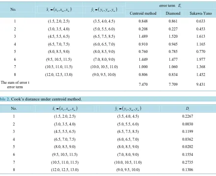
[image:6.595.141.487.435.712.2]By formula (7), we calculate the model’s error term Ei and it’s sum using centroid method, Diamond’s me-thod and Sakawa-Yano’s meme-thod, and the results are listed in Table 1. From Table 1, we can find that the sum of the model’s error term using centroid method is less than using Diamond’s method and Sakawa-Yano’s me-thod. Thus, the result of fuzzy linear regression model using centroid method is better than using Diamond’s method and Sakawa-Yano’s method.
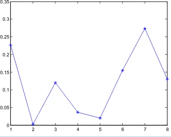
Figure 1obtained by Matlab programming.
Table 2 and Figure 1 show Cook’s distance under centroid method and their scatter plot, respectively. Be-cause of being with the Cook’s distance. These results indicate that the data point No. 7 is an outlier or strong impact point.
Figure 1. The scatter plot of Cook’s distance under centroid method.
1 2 3 4 5 6 7 8
Table 1. Data from Sakawa and Yano [15].
No. xi=(x xil, im,xiu) yi=(yil,yim,yiu)
error term Ei
Centroid method Diamond Sakawa-Yano
1 (1.5, 2.0, 2.5) (3.5, 4.0, 4.5) 0.848 0.861 0.633
2 (3.0, 3.5, 4.0) (5.0, 5.5, 6.0) 0.208 0.227 0.453
3 (4.5, 5.5, 6.5) (6.5, 7.5, 8.5) 1.489 1.520 1.613
4 (6.5, 7.0, 7.5) (6.0, 6.5, 7.0) 0.910 0.945 1.165
5 (8.0, 8.5, 9.0) (8.0, 8.5, 9.0) 0.760 0.785 0.770
6 (9.5, 10.5, 11.5) (7.0, 8.0, 9.0) 1.449 1.477 1.977
7 (10.5, 11.0, 11.5) (10.0, 10.5, 11.0) 1.000 1.060 1.368
8 (12.0, 12.5, 13.0) (9.0, 9.5, 10.0) 0.806 0.834 1.452
The sum of error t
[image:7.595.97.537.98.457.2]error term 7.470 7.709 9.431
Table 2. Cook’s distance under centroid method.
No. xi=(x xil, im,xiu) yi=(yil,yim,yiu) Di
1 (1.5, 2.0, 2.5) (3.5, 4.0, 4.5) 0.2267
2 (3.0, 3.5, 4.0) (5.0, 5.5, 6.0) 0.0030
3 (4.5, 5.5, 6.5) (6.5, 7.5, 8.5) 0.1199
4 (6.5, 7.0, 7.5) (6.0, 6.5, 7.0) 0.0362
5 (8.0, 8.5, 9.0) (8.0, 8.5, 9.0) 0.0202
6 (9.5, 10.5, 11.5) (7.0, 8.0, 9.0) 0.1554
7 (10.5, 11.0, 11.5) (10.0, 10.5, 11.0) 0.2735
8 (12.0, 12.5, 13.0) (9.0, 9.5, 10.0) 0.1306
6. Conclusion
By transforming fuzzy data into clear data, the fuzzy linear regression model is transformed into traditional li-near regression model. We study the parameter estimation and impact analysis of the case-deletion fuzzy lili-near regression model. By comparing with other methods through a practical example, we can conclude that the pro-posed method in this paper can be used easily and have a good fitting performance.
Acknowledgements
This research is supported by National Natural Science Foundation Grant No. 11171065, the National Statistical Scientific Foundation Grant No. 2014LY059.
References
[1] Zadeh, L.A. (1975) The Concept of Linguistic Variable and Its Application to Approximate Reasoning. Information Sciences, 8, 99-244, 301-357.
[2] Thanaka, H., Uejina, S. and Asai, K. (1982) Linear Regression Analysis with Fuzzy Model. IEEE Trans Systems Man Cybernetics, 12, 903-907.
[3] Diamond, P. (1988) Fuzzy Least Squares. Information Science, 46, 141-157.
http://dx.doi.org/10.1016/0020-0255(88)90047-3
[4] Savic, D.A. and Pedrycz, W. (1988) Evaluation of Fuzzy Linear Regression Models. Fuzzy Sets and Systems, 46, 141- 157.
Systems, 119, 225-246. http://dx.doi.org/10.1016/S0165-0114(99)00092-5
[6] Kim, B. and Bishu, R.R. (1998) Evaluation of Fuzzy Linear Regression Model by Comparison Membership Function. Fuzzy Set and Systems, 100, 343-352. http://dx.doi.org/10.1016/S0165-0114(97)00100-0
[7] Nasrabadi, M.M. and Nasrabadi, E. (2004) A Mathematical-Progrmming Approach to Fuzzy Linear Regression Analy-sis. Applied Mathematics and Computation, 155, 873-881. http://dx.doi.org/10.1016/j.amc.2003.07.031
[8] Kao, C. and Chyu, C.L. (2002) A Fuzzy Linear Regression Model with Better Explanatory Power. Fuzzy Sets and Sys-tems, 126, 401-409. http://dx.doi.org/10.1016/S0165-0114(01)00069-0
[9] Yeh, C.-T. (2011) A Formula for Fuzzy Linear Regression Analysis. 2011 IEEE International Conference on Fuzzy Systems, Taipei, 27-30 June 2011, 2845-2850.
[10] Azadeh, A., Neshat, N. and Rafiee, K. (2015) An Adaptive Neural Network-Fuzzy Linear Regression Approach for Improved Car Ownership Estimation and Forecasting in Complex and Uncertain Environments: The Case of Iran. Transportation Planning and Technology, 35, 221. http://dx.doi.org/10.1080/03081060.2011.651887
[11] Yager, R.R. (1980) On a General Class of Fuzzy Connectives. Fuzzy Set and Systems, 4, 235-242.
http://dx.doi.org/10.1016/0165-0114(80)90013-5
[12] Chen, S.J. and Hwang, C.L. (1992) Fuzzy Multiple Attribute Decision Making. Springer, NY.
http://dx.doi.org/10.1007/978-3-642-46768-4
[13] Wei, B.C., Lin, J.G. and Xie, F.C. (2009) Diagnostic Statistics. Higher Education Press, Beijing, 19-44. [14] Cook, R.D. (1977) Detection of Influential Observations in Linear Regression. Technometrics, 19, 15-18.
http://dx.doi.org/10.1080/00401706.1977.10489493