Open Journal of Social Sciences, 2014, 2, 64-71
Published Online January 2014 in SciRes
Dealing with Model Mis-Specification in the
Analysis of Morale in Old Age
Said Shahtahmasebi1,2,3 1Centre for Health and Social Practice, Wintec, New Zealand2The Good Life Research Centre Trust, New Zealand 3Division of Adolescent Medicine, Department of Pediatrics, Kentucky Children’s Hospital,
University of Kentucky, Lexington, USA
Received 9 August 2013; revised 10 September 2013; accepted 17 September 2013
Copyright © 2014 Said Shahtahmasebi. This is an open access article distributed under the Creative Commons Attribution License, which permits unrestricted use, distribution, and reproduction in any medium, provided the original work is properly cited. In accordance of the Creative Commons Attribution License all Copyrights © 2014 are reserved for SCIRP and the owner of the intellectual property Said Shahtahmasebi. All Copyright © 2014 are guarded by law and by SCIRP as a guardian.
Abstract
A major challenge for analysis of data from observational and survey studies is dealing with model mis-specification. A common reason for model mis-specification is the violation of the independence assumption. Model mis-specification is frequently due to the inclusion of variables that are corre-lated with the error terms (serial correlation) or due to variables omitted from the study. The appli- cation of standard regression models to such data could lead to over inflated results, i.e. erroneous results, and misleading conclusions. Longitudinally designed studies make substantial improve- ments and provide an additional handle to control omitted variables. However, even with longitu- dinal data, model mis-specification could occur because of the nature of observations, i.e. surveys often include objectively as well as subjectively measured variables. Subjective variables are respon- sible for model mis-specification, therefore, compounding the problem further. One solution to such problems is the application of instrumental variables. The instrumental variable method is seldom used with social survey data. The main criticism is the arbitrary selection of variables as instruments. Longitudinal data, because of its temporal structure, provide natural instruments. In this paper, a pragmatic strategy for analysis is proposed that utilises the nature of the data (subjective/objective) and a combination of methods within a longitudinal modelling framework to correct for model mis- specification. These applications are illustrated by using recurrent continuous morale in old age from a longitudinal survey of the elderly. The results suggest a strong presence of heterogeneity effect, i.e.
current levels of morale appear to be individual-specific and independent of its previous levels.
Keywords
1. Introduction
As more people are expected to live longer, quality of life in old age has been one of the main focuses for re- search and policy development. Quality of life, happiness, positive aging, life satisfaction, and so on, have been linked to health and overall wellbeing (e.g. see [1-6]). This is particularly important for the elderly who live in isolation or in rural areas. Social isolation may not necessarily be due to geographical distance between elderly people and their support network, it could well be due to the size of their social support network [7]. Morale in old age is an important concept and has been used as an indicator of overall wellbeing and quality of life in old
age [1-6]. The assumption is that changes in morale could affect changes in well-being (e.g. see [2]). However,
the question that arises is: does high morale lead to a perception of good health and therefore higher quality of life, or, does good health and higher quality of life lead to higher morale in old age (past behaviour effect)? Mo- rale, and in general quality of life are complex concepts and are subjective in nature which have implications for defining, measuring and analysing them [8]. The aim of this paper is to demonstrate problems arising from studying such complex concepts and illustrate an analytical strategy not only to anticipate but also to overcome problematic issues. Unfortunately, despite advancement in software technology and statistical modelling, model mis-specification is still a big problem when dealing with observational data. In this context, morale in old age provides an excellent example.
Issues relevant to studying morale in old age were discussed in earlier papers [9-11] which highlighted prob- lems measuring and modelling quality of life variables. One of the fundamental methodological problems, quite apart from the issues of defining and measuring quality of life, is disentangling the complex inter-relationships between quality of life and other variables. As with any research based on survey data, it is difficult to distin- guish systematic patterns from random ones due to other variables. The flexibility of survey/observational stud-ies to measure a wide range of subjective and objective variables adds complexitstud-ies to analyses. Survey studstud-ies of elderly people living in the community do not often include measures of depression, morale or dementia all at the same time. In this context, quite apart from the methodological issues of multicollinearity and the direction of causality, the issue of bias in the sample, due to unmeasured or omitted variables, needs also to be addressed. Furthermore, the adopted statistical modelling must be able to handle past behaviour effect (e.g. state depend- ence) and heterogeneity effect due to omitted variables (e.g. frailty).
Heterogeneity results when systematic but unmeasured characteristics of individuals contribute to response patterns over time. In survey studies, some individual characteristics are often omitted either because they are unobserved or difficult to measure. Omitted characteristics such as frailty, could lead to spurious relationships between the observed characteristics and the outcome variables. Past behaviour effect exists when the experi-ence of a particular outcome itself changes the probability of experiencing that event on subsequent occasions. Again, it is clear that past behaviour cannot be addressed within cross-sectional designs. Heterogeneity and past behaviour effects are common when dealing with behavioural data, and ignoring them will produce bias in vari-ability estimates and tests of treatment related with hypothesis [12,13]. Although these issues can be addressed with the application of advanced statistical modelling, these models cannot account for additional complexities in data, due to temporal dependencies, simultaneously.
This paper identifies some of these problematic issues when analysing longitudinal data on quality of life in old age and describes a statistical modelling strategy to address the various problems simultaneously.
2. Methods
In this paper a secondary data source (the rural North Wales Elderly Project) is used in order to demonstrate the complexities arising from analysis of data from observational studies.
As mentioned above, there have been numerous studies of aging (e.g. [2,14]. The main interest of these stud- ies is to observe changes in individuals’ circumstances over time and to examine any possible link with an out- come of interest e.g. health, longevity. The Rural North Wales Elderly Project [15] extended the investigation of the ageing process to individuals’ social activities and social interaction. Social networks, other quality of life measures (e.g. morale, loneliness and social isolation), and how they may vary over time with age and life events (e.g. bereavement, dependency) are prominent features of such studies.
questionnaire [15]. In 1984, the project was repeated on a sub-sample surveying only those who were age 75 and over in 1979. In 1987 the project was repeated and surveyed all surviving members of the original sample. This provided a slightly staggered longitudinal study in old age, i.e. three time-point measures (1979, 84, 87) are only available for the old elderly, and two-time point measures for the whole sample are only available at baseline (1979) and in 1987 (see [9]). Some additional measures using a much shorter version of the questionnaire be- came available in 1991 and 1995. A wide range of topics were included in the survey including demography, socio-economic, social activities and contacts, health, life events, attitudes to life and so on.
As well as demographic and socio-economic measures, the data set is rich in various measures on quality of life (e.g. morale, loneliness, companionship, hours spent alone, social contact, supportive network), dependency (e.g. self-assessed health, long-standing illness, mobility, hours spent alone, supportive network), survival (e.g. dates of death, duration survived, trace variables), health care and service use (e.g. use of district nurse, GP, home help) and informal support (e.g. relatives, friends and neighbours). Therefore, analyses can be designed to investigate quality of life in old age in the context of, for example, supportive networks of the elderly people, morale in old age, loneliness in old age, health, mobility, migration and housing in old age (see [16]).
One of the topics of interest in this survey was morale in old age; “what factors govern morale in old age”. Given the structure of the data set a number of strategies for analyses were developed and carried out e.g. see [9,11].
In this paper, I report on a strategy for analysis that allows simultaneous control for past behaviour and het- erogeneity while at the same time enables handling of model mis-specification due to a complex unforeseen re- lationship between observed and omitted variables. For this analysis, data from the interval 1983-87 is used for the main reasons that, first, a number of dependency measures are only available in the 1983 and 1987 question- naires and were not asked in 1979, and second, this strategy allows the inclusion of past behaviour in the analysis.
Substantive issues: From the literature review [10,11] a large number of socio-economic, health, environ- mental and individual variables can be associated with morale in old age. Therefore multicollinearity is one of the important issues to be considered in any strategy for analysis.
An important substantive question is the dynamics of morale in old age, i.e. does it fluctuate according to a change in variables, or, whether morale level remains constant (past behaviour)?
Furthermore, survey questionnaires provide two main challenges with data; omitted variables and subjectivity. Surveys often exclude and omit variables because they are either unmeasureable or difficult to measure, e.g. frailty or the feel good factor.
On the other hand, surveys frequently use self-assessment tools to measure social, health and individual vari-ables such as state of health and emotional wellbeing. Subjective varivari-ables, therefore, carry measurement errors that can contribute to model mis-specification; subjectivity is responsible for erroneous results [9].
Thus, the analytical strategy must be modified to allow simultaneous statistical control for multicollinearity, past behaviour, omitted variables and subjectivity.
Response variable: The anglicised version of Philadelphia Geriatric Centre Morale Scale [9,11] was used, as part of the survey questionnaire, to measure morale in old age. This is a continuous scale taking values (1.0 - 3.0) with 1.0 measuring low morale sliding up to 3.0 high morale. There are 38 cases with a valid morale score at each interval point 1983 and 1987 in the North Wales Elderly data.
Explanatory variables: A large number of variables, including those reported in the literature, were extracted from the main data set and included in the analysis (see Appendix). As mentioned above, subjectivity is an im- portant issue so explanatory variables were distinguished as subjective and objective variables. Variables were classed as subjective if they were reflecting a perception or self-assessment such as “self-reported health”, “peo- ple in the area they could call friends”, otherwise classed as objective such as “number of children”, “having close relatives”, “age”.
0 1
for time=1983 yit =β +γyit− +βxit+ +θ εi it (1)
1 0 1 1
for time=1987 yit+ =β +γyit+βxit+ + +θ εi it+ (2)
where γyit−1 is the dummy variable for the past behaviour and θ is the time constant individual specific error term. The error terms are assumed to be independent of the {x}. This model could be fitted to data using condi- tional or marginal likelihood method [9,17-19]}. The application of marginal likelihood method to this data has been demonstrated in an earlier paper, see [9].
Conditional likelihood method: This paper reports the results from the application of the conditional like- lihood method, sometimes referred to as the difference method. The conditional method detect change by sub- tracting Equation (1) from Equation (2)
(
)
(
) (
)
1 1 1 1
it it it it it it it it
y+ −y =γ y −y − +β x+ −βx + ε + −ε (3)
thus eliminating θ and all other time constant variables such as sex. This model can be fitted using any statis- tical packages such as STATA and SAS, for this analysis GLIM4 was used and results are shown in Table 1
column headed “conditional”.
Unexpected results: The result (see Table 1 column headed “conditional”) suggests that past behaviour is highly significant and that previous low morale is significantly related to current high morale! Having explicitly expressed the difference equation in terms of all the elements is relatively easy to identify the source of the problem. It is fairly obvious that fitting this model to the data will lead to a well known specification problem. The problem is due to the violation of the independence assumption: the dummy variable for past behaviour contains an element (yit) that is associated with the error term on the same side of the equation. This model was
nevertheless fitted to data to demonstrate the impact on result.
Solution: The problem where one or more explanatory variables are associated with the error term is also
[image:4.595.172.426.449.696.2]known as errors-in-variables or serial correlation. This is a common but rarely addressed problem in behavioural sciences, in particular with observational studies, as both objective and subjective variables are used as inde- pendent variables. The solution is the application of instrumental variables method, where the offending vari- able(s) are replaced by another or a set of variables that have no association with the error term but are highly correlated with the offending variables. Identifying variables as instruments can be a major issue.
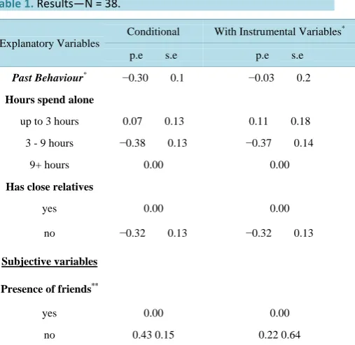
Table 1.Results—N = 38.
Explanatory Variables
Conditional With Instrumental Variables*
p.e s.e p.e s.e
Past Behaviour* −0.30 0.1 −0.03 0.2
Hours spend alone
up to 3 hours 0.07 0.13 0.11 0.18
3 - 9 hours −0.38 0.13 −0.37 0.14 9+ hours 0.00 0.00
Has close relatives
yes 0.00 0.00
no −0.32 0.13 −0.32 0.13
Subjective variables
Presence of friends**
yes 0.00 0.00
no 0.43 0.15 0.22 0.64
*
Fortunately, data sets with a longitudinal structure can provide natural and logical instrument. For Equation (3), the best instrument is morale measured at pre 1983 time point, i.e. at 1979 (baseline) [17]. HUMMER [20]
was used to fit the model with morale in 1979 as an instrument for past behaviour. The result, suggests that this variable is no longer significant which means that, at least with this data, morale in old age is not influenced by its own past levels.
3. Results
The variable past behaviour is dropped from the model. Model selection continues with the remaining explana- tory variables. The forward substitution method was used for model selection. The final model is shown in Ta- ble 1 and includes two objective variables (hours spent alone, and has close relatives), and only one subjective variable (presence of friends in the area). Model fitting results (parameter estimates and standard errors) are shown in Table 1 (column headed “conditional”). Looking at the remaining results after dropping past behav- iour it can be seen that the only remaining subjective variable is highly significant, but, with a counter intuitive effect; those who claimed that they had no friends in the area appear to score higher on the morale scale than those who said they had.
This counter intuitive result may well be due to the errors-in-variables problem mentioned above, where the subjective variable ‘presence of friends’ is correlated with the error term. As explained above the solution to this problem is the application of instrumental variables method. Objective variables already selected in the model are not correlated with the error term, so a logical choice of instrument(s) is to use the objective variables as in- struments for the subjective variable.
The results for fitting the new model with instruments are shown in the second column of Table 1. It can be seen that, after correcting for mis-specification, this variable is no longer significant. Models without corrections for omitted variables and measurements error lead to an under-estimation of standard errors and over inflated parameter estimates thus a false high statistical significance level [20,21]. Therefore, an increase in the standard error of the subjective variable can be noticed after correcting for residual heterogeneity (q) and errors-in-vari- ables. The large reduction in the parameter estimate of the variable “presence of friends” indicates possibly more complex interactions in data.
It can also be noticed that there is no or very little change in the parameter estimates and standard errors of the objective variables with or without instrumental variables. The results for the objective variables are fairly straight forward; those who claimed spending between 3 - 9 hours alone appear to do worse on the morale scale. This group of elderly people appear to be more dependent, less mobile and require more looking after. Those who do not have any close living relatives appear to do worse than those who claimed they had a living close relative.
4. Implication for Theory
As demonstrated by the analysis of a real world data set above, complex inter-relationships in observational data can make analysis of such data more challenging. A longitudinal study design together with appropriate longitu- dinal model (such as model in Equation (1)) may help meet some of the challenges. Often a time constant va- riance component
( )
θi is specified where in fact a model with a time varying variance component should befitted to data, e.g.
0
it it i it it
y =β +βx + +θ ξ +ε (4)
where θi is the individual specific (time constant omitted variables), xit is time varying omitted variables, and
it
ε is the structural error term. This model cannot be estimated because of too many unknowns. However, the analysis of morale in old age using conditional likelihood method and instrumental variables method reported above suggests a pragmatic approach to fit such a model to data.
Consider re-writing Equation (3) whilst distinguishing subjective variables
{ }
x′ from the objective variables {x}:(
)
(
) (
)
1 1 1 1
it it it it it it it it
y+ −y =β x+ −x +β′ ′x+ −x′ + ε + −ε (5)
it it it
x′ = x′∗+ε′
where xit ∗
′ is the unobserved true value of subjective variables and εit is measurement errors. Rewriting Equ-
ation (5) in terms of the true value of subjective variables:
(
)
(
* *)
(
) (
)
1 1 1 1 1
it it it it it it it it it it
y+ −y =β x + −x +β′ ′x+ −x′ +β ε′ ′+ −ε′ + ε + −ε (6)
or
(
*)
it it it it i it
y =βx +β′ ′x +ε′ + +θ ε (7)
The models in Equations (6) & (7) are indeed equivalent to the desired model expressed in Equation (4). The model in Equation (6) & (7) cannot be fitted because the actual values for
{ }
*x′ are unknown. However, as demonstrated in Table 1 (and Equation (3)) the model in Equation (6) was fitted using the observed values of the subjective variables, i.e. the set of x′, and the instrumental variables method to account for possible mea- surement error, and the conditional likelihood method to control for θ: i.e. a pragmatic approach of fitting models of the following type:
0
it it i it it
y =β +βx + +θ ξ +ε
where θi is the individual specific (time constant omitted variables) i.i.d error term, ξit time varying omitted
variables i.i.d error term and εit is the structural i.i.d error term.
5. Conclusions
In the final analysis, it appears that the variable “presence of friends” must have owed its significance to its rela- tionship with other factors omitted from the analysis. The results reported do tend to emphasize the complexity of the task of developing parsimonious models when there is high multicollinearity between variables both ob- served and unobserved.
The use of the conditional likelihood method, together with instrumental variables allows control for time- variant omitted variables simultaneously with other structural and nuisance parameters.
The results shown in the second column of Table 1, after controlling for time-variant omitted variables, sug- gest that the subjective variables are no longer significant. Moreover, the results can be interpreted as low mo- rale being associated with physical dependence on “others”, while the availability of, or (both physical and men- tal) dependence on close relatives including spouse may lead to high morale in old age.
Finally, because of more extensive control, the final analyses (conditional likelihood with instrumental vari- ables methods) have more authority. An additional advantage with the final analyses over the conditional likely- hood method is to allow the inclusion of time-invariant factors in the modelling process. For example, the ef- fects from time-constant variables such as sex could be controlled for after differencing by using such variables as instruments for subjective variables which are known to carry measurement error.
Acknowledgements
Based on the research conducted by Professor Clare Wenger and jointly funded by the Department of Health and Social Security/Welsh Office and Economic and Social Research Council (G00212334), the analysis reported in this paper was carried out during the author’s employment at the Centre for Social Policy Research and De- velopment (CSPRD), University of Wales, Bangor.
An earlier version of this paper was presented at the 8th International Conference on Social Science Method- ology (RC33), July 9th-13th, 2012, Sydney, Australia.
References
[1] Moser, C., Spagnoli, J. and Santos-Eggimann, B. (2011) Self-perception of aging and vulnerability to adverse out- comes at the age of 65 - 70 years. The Journals of Gerontology Series B: Psychological Sciences and Social Sciences, 66, 675-680
[3] Hassel, A.J., et al. (2011) Oral health-related quality of life is linked with subjective well-being and depression in early
old age. Clinical Oral Investigations, 15, 691-697.
[4] Cho, J., et al. (2011) The relationship between physical health and psychological well-being among oldest-old adults. Journal of Aging Research, 2011, Article ID: 605041.
[5] Ailshire, J.A. and Crimmins, E.M. (2011) Psychosocial factors associated with longevity in the United States: Age dif-ferences between the old and oldest-old in the health and retirement study. Journal of Aging Research, 2011, Article ID: 530534
[6] Deng, J., et al. (2010) Subjective well-being, social support, and age-related functioning among the very old in China.
International Journal of Geriatric Psychiatry, 25,
697-[7] Wenger, G.C., et al. (1996) Social isolation and loneliness in old age: Review and model refinement. Ageing and
Soci-ety, 16, 333-358.
[8] Fernández-Ballesteros, R. (2011) Quality of life in old age: Problematic issues. Applied Research in Quality of Life, 6,
21-[9] Shahtahmasebi, S. (2004) Quality of life: A longitudinal analysis of correlates of morale in old age. The Scientific
World Journal, 4, 100-110
[10] Wenger, G.C. (1992) Morale in old age: A review of the literature. International Journal of Geriatric Psychiatry, 7, 699-708.
[11] Wenger, G.C., Davies, R. and Shahtahmasebi, S. (1995) Morale in old age: Refining the model. International Journal
of Geriatric Psychiatry, 10,
933-[12] Davies, R.B. (1987) The limitation of cross-sectional analysis. In: Crouchley, R., Ed., Longitudinal Data Analysis, Sage, London.
[13] Gibbons, R.D., et al. (1993) Some conceptual and statistal issues in analysis of longitudinal psychiatric data: Applica-tion to the NIMH Treatment of Depression Collaborative Research Program dataset. Archives of General Psychiatry, 50, 739-750
[14] Litwin, H. and Shiovitz-Ezra, S. (2011) Social network type and subjective well-being in a national sample of older
Americans. The Gerontologist, 51, 379-388.
[15] Wenger, G.C. (1984) The supportive network—Coping with old age. George Allen and Unwin, London.
[16] Shahtahmasebi, S. and Berridge, D. (2010) Conceptualising behaviour in health and social research: A practical guide to data analysis, ed. J. Merrick. Nova Sci, New York.
[17] Anderson, T.W. and Hsiao, C. (1981) Estimation of dynamic models with error components. American Statistics Asso-ciation, 76, 375.
[18] Chamberlain, G. (1980) Analysis of covariance with qualitative data review of economic studies. XLVII, 225-238.
[19] Davies, R., Martin, A.M. and Penn, R. (1988) Linear modelling with clustered observations an illustratative example of earnings in the engineering industry. Environment and Planning A, 20,
1069-[20] Wallace, D. and Silver, J.L. (1988) Econometrics—An introduction. Addison-Wesley, New York.
[21] Pickles, A.R. and Davies, R.B. (1989) Inference from cross-sectional and longitudinal data for dynamic behavioural processes. In: Hauer, J., Ed., Urban Dynamics and Spatial Choice Behaviour, Kluwer Academic, 49, 81-104.
Appendix.List of explanatory variables.
Age Continuous
Sex Male, female
Income Low: up to £39, £40 - £79; comfortable: £80 - £99; above average: £100+
Social class Class I, II/III, IV/V
Home tenure Owner occupier, local authority rented accommodation, private rented, other (for the old elderly sample; owner occupier, rented, other)
Ethnicity Welsh, Non-Welsh
Marital status Single, married, widowed, divorced/separated
Social support variables
Frequency see family Every day, at least weekly, at least monthly, less often, never/no relatives
Relative seen most often No relatives, child, sibling, other
Who cares when ill Spouse, relative in/out house, friend/neighbour, other, no one/d/k/missing—was used for 1979 cross-sectional analysis only
Network type Family dependent, locally integrated, local self-contained, wider community focused, private restricted
Loss variables
Change in marital status No change, lost spouse, married—1983 and 1987 intervals only
Number of years widowed Continuous
Health
Housebound Yes, no
Self-assessed health Subjective; excellent/good, alright for age, fair/poor
Health-limited activities Subjective; yes, no
Isolation variables
Household composition Lives alone, with spouse, with others
Has close relative(s) Yes, no
Visits relatives At least weekly, at least 6/year, less often, no relatives/never
Has telephone Yes, no
Nearest neighbour Next door attached/det., across road/50 - 100 yards, 100+ yards
Hours spent alone 0 - 3 hours/day, 3 - 9 hours/day, 9+ hours/day
Isolation measure Continuous—a combination of 7 objective variables reflecting social contact
Loneliness variables
People available to do favours Subjective; yes, no, never ask favours
Presence of real friends Subjective; yes, no—respondent were asked to list names
Wish for more friends Subjective; yes, no
Confidant Subjective; no one, spouse, other
Self-assessed loneliness Subjective; never/rarely, sometimes, often/always