An Efficient Storage Format for Large Sparse Matrices based on Quadtree

An Efficient Storage Format for Large Sparse Matrices

based on Quadtree

Nidhal K. El Abbadi Elaf J. Al Taee

University of Kufa University of Kufa Najaf, Iraq Najaf Iraq

ABSTRACT

There are serious problem for storage sparse matrix due to west of memory used for storage the non-zero values which represent more than 90% of sparse matrix. There are many algorithms suggested for solving this problem.

A new storage method for large sparse matrices was presented in this paper based on quadtree. The suggested algorithm utilized the idea of quadtree to re-represent the sparse matrix in two vectors, which reduce the required memory space for storage sparse matrix. The suggested algorithm reduced the memory space required to store the zero values to more than 85%. The algorithm compared with many algorithms and it was more efficient than almost all the previous algorithms up to our knowledge. The current algorithm characterized by less space storage need, highly speed, and easy to implement.

Keywords

Sparse matrix, quadtree, compression, decompression

1.

INTRODUCTION

A sparse matrix defined as a matrix, which has very few nonzero elements, while a dense matrix defined as a matrix, which has very few zero elements.

Sparse matrices (matrices with a substantial minority of non-zero elements, normally less than 10% non-non-zero elements) are pervasive in many mathematical and scientific applications. These matrices provide an opportunity to minimise storage and computational requirements by storing, and performing arithmetic with, only the non-zero elements. The many existing formats for sparse matrices are derived from different means of taking advantage of sparsity patterns in frequently occurring matrices [1].

A sparse matrix is seems worthwhile to use a more space efficient data structure to store it than a simple two dimensional array. Space efficient data structures for sparse matrices try to store only the nonzero elements. This results in considerable savings in space for the matrix elements and time for operations on them, at the cost of some space and time overhead to keep the data structure consistent.

The natural idea to take advantage of the zeros of a matrix and their locations was initiated by engineers in various disciplines. In the simplest case involving banded matrices, special techniques are straightforward to develop. Electrical engineers dealing with electrical networks in the 1960s were the first to exploit sparsity to solve general sparse linear systems for matrices with irregular structure. The main issue, and the first addressed by sparse matrix technology, was to devise direct solution methods for linear systems. These had to be economical, both in terms of storage and computational effort. Sparse direct solvers can handle very large problems that cannot be tackled by the usual "dense" solvers [2].

Essentially, there are two broad types of sparse matrices: structured and unstructured. A structured matrix is one whose nonzero entries form a regular pattern, often along a small number of diagonals. Alternatively, the nonzero elements may lie in blocks (dense sub-matrices) of the same size, which form a regular pattern, typically along a small number of (block) diagonals. A matrix with irregularly located entries is said to be irregularly structured.

The recursive decomposition of a complex problem into simpler sub-problems, known in the literature as the divide-and-conquer paradigm, is a well-practiced technique for solving many computational problems has successfully employed such techniques for 2-dimensional data representation. Their technique recursively decomposes the original data area of square shape into four identical squares at each step. The resulting data structure represents a quadtree [3].

Quadtree matrix representation has been recently proposed as an alternative to the conventional linear storage of matrices. If all elements of a matrix are zero, then the matrix is represented by an empty tree, otherwise it is represented by tree consisting of four sub-trees, each representing, recursively, a quadrant of the matrix. Using four-way block decomposition, algorithms on quadtrees accelerate on blocks entirely of zeroes, and thereby offer improved performance on sparse matrices [4].

There exists a large number of storage formats algorithms for sparse matrices, such as the compressed row format, compressed column format, block compressed row storage, compressed diagonal storage, jagged diagonal format, transposed jagged diagonal format and skyline storage. The Sparskit library supports 16 different sparse matrix formats. These storage formats are designed to take advantage of the structural properties of sparse matrices, both with respect to the amount of memory needed to store the matrix and the computing time to perform operations on it [5].

2.

QUADTREE

Hierarchical data structures are important representations in the domains of computer vision, robotics, computer graphics, image processing, pattern recognition, and geographic information systems. One such data structure is the quadtree.

Today, the term quadtree is used in a general sense to describe a class of data structures whose common property is that they are based on the principle of recursive decomposition of space.

parent node and can have any number of children nodes, including zero.

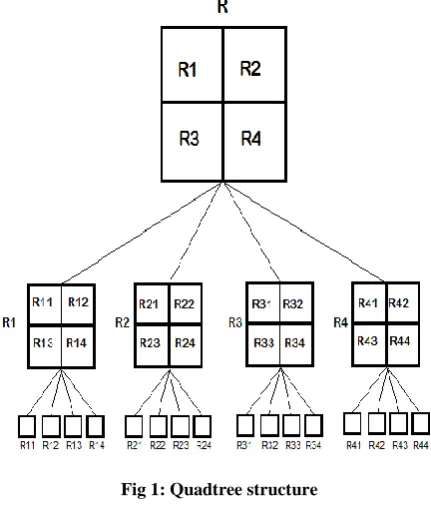
Unlike a normal tree data structure, a quad tree structure requires that each internal node have exactly four children nodes. When illustrating most quad tree structures, you'll see a node that has four children nodes hanging from it, with lines connecting the parent node with its children nodes. The illustration can continue, with four more children nodes hanging from each of the original four children nodes as shown in Fig. 1.

Other times, the illustration of a quad tree will be a region or square. Whenever the region reaches its maximum capacity for storing data, it is divided into four quadrants. Normally, the regions and the quadrants are squares, although they can be rectangles or other shapes, too.

There are two restrictions of quadtrees, the first one is large memory storage space needed and the second one is the representation of object based on its location, orientation, and relative size. The quadtree data structure needs many pointers and these pointers need more storage space, non terminal node need five pointers [3].

Fig 1: Quadtree structure

3.

METHODOLOGY

The main idea considered in compressed storage formats is to avoid the handling and storage of zero values in irregular sparse matrix. This is accomplished by means of the storage of the non-zero elements of the sparse matrix in a contiguous way using a linear array. However, some additional arrays are needed for knowing where the non-zero elements fit into the sparse matrix. The number of subsidiary arrays varies depending on the storage format used.

The current research presents simple and efficient algorithm to represent the sparse matrix with minimum size. The suggested algorithm based on quadtree. Algorithm consists mainly of two parts, the compression part of sparse matrix and the decompression part.

3.1

Compression or Storage Format of

Sparse Matrix

The input matrix is sparse matrix (most of the elements are zero) with few elements are non-zero distributed randomly in the matrix. To compress this matrix we suggested to make the matrix square with equal dimensions size (dimension as power of two), this will simplified the work, and adding zero in row or column to make dimensions equal and power of two, will not effect on the matrix and it is easy to eliminate later after decompression.

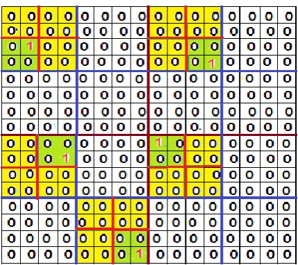
The suggested algorithm suggested two vectors, one to carry the non-zero values called values vector, while the other hold the values represent the matrix structure called the structure vector. Fig 2 shows the suggested matrix (16 × 16) with 2% non-zero value to help us explaining the suggested algorithm.

Fig 2: suggested sparse matrix

The sparse matrix scanned from left to right and top to down. Each non-zero value shift to the values vector and insert one instead of it in sparse matrix Fig 3 shows the resulted matrix.

Fig 3: sparse matrix after removing the non-zero values.

Values vector = [9, 22, 23, 54, 12]

Fig 4: sparse matrix after dividing it to four parts

Structure vector = [1, 1, 1, 1]

This process of quad tree continue to dividing each part has value one in the structure vector to four parts, for our example all the four parts in Fig 4 will be divided to four parts for each as showed in Fig 5.

Fig 5: dividing the parts with value one in structure vector to four parts each.

The same thing we did for the new matrix insert one or zero in the structure vector according to values of each part in the corresponding part of sparse matrix. The updated structure vector becomes:

Structure vector = [1, 1, 1, 1, 1, 0, 0, 0, 1, 0, 0, 0, 1, 0, 0, 1, 1, 0, 0, 0]

This process continues until the dimension of each part equal to 2. In the current example, we need one more dividing just for each part has the corresponding value one in the structure vector, the result showed in Fig 6.

Fig 6: more dividing for sparse matrix for parts with value one in the structure vector.

The structure vector will be updating according to new matrix in Fig 6 (always the values (zero or one) for the new parts resulted from dividing part/s with value one in the structure vector will be added to the structure vector).

Structure vector = [1, 1, 1, 1, 1, 0, 0, 0, 1, 0, 0, 0, 1, 0, 0, 1, 1, 0, 0, 0, 0, 0, 1, 0, 0, 0, 0, 1, 0, 1, 0, 0, 0, 0, 0, 1, 1, 0, 0, 0]

When the dimension of each part equal 2, then the last step in quadtree process implemented. The value of each part has one cell or more equal one will be added to the structure vector (at this case all the part value added with the same way of quad tree. For example, part 1 in the figure 6 which has one cell with value one (the other parts are zero values) will be written in the structure vector as follow:

= (0, 1, 0, 0)

According to that, the structure vector updated to become (color to represent each level of process):

Structure vector = [1, 1, 1, 1, 1, 0, 0, 0, 1, 0, 0, 0, 1, 0, 0, 1, 1, 0, 0, 0, 0, 0, 1, 0, 0, 0, 0, 1, 0, 1, 0, 0, 0, 0, 0, 1, 1, 0, 0, 0, 0, 1, 0, 0, 0, 0, 0, 1, 0, 0, 0, 1, 0, 0, 0, 1, 1, 0, 0, 0]

The last step in compression process is to re-represent the structure vector. The structure vector looks as a vector of binary values, for that it is easy to rewrite it as a vector of decimal values. Each 8 consequent values in the structure vector converted to corresponding decimal value. The result will be as follow:

Structure value= [248, 137, 130, 20, 24, 65, 17, 8]

At this case, one byte used to store each value.

3.2

Decompression process

The decompression process is almost the inverse of compression process. We start with the structure vector to rebuild the matrix structure. Convert the decimal value of structure vector to binary value.

Then the size of matrix = ( 2 )level

After we find the size of matrix then we use the values in the values vector to insert in the matrix instead of the value one at the same order from left to right and top to down. The last step is to insert the value in the value vector instead of each element with value one in the resulted matrix, this done by scanning the resulted matrix from left to right and top to down.

4.

THE RESULTS

1. The compression ratio for the current proposal was measured, this done for different matrix size and different percent of non-zero value ranged from 1% to 10% for each matrix size. Fig 7 showed the results.

Fig 7: compression ratio for various matrices size and various percent of non-zero values.

2. Measuring the time needed for compression the sparse matrix, again we check for different matrix size and non-zero value ranged from 1% to 10% for each matrix size. The result showed in Fig 8.

Fig 8: compression time for various matrices size and various sizes of non-zero values

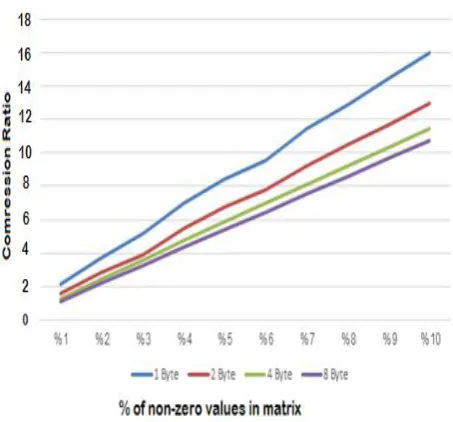
3. The compression ratio for the sparse matrix checked when each value in sparse matrix represented with one or more than one byte, as showed in figure 9 and Fig 10.

compression ratio = _{𝑠𝑖𝑧𝑒 𝑏𝑒𝑓𝑜𝑟𝑒 𝑐𝑜𝑚𝑝𝑟𝑒𝑠𝑠𝑖𝑜𝑛}𝑠𝑖𝑧𝑒 𝑎𝑓𝑡𝑒𝑟 𝑐𝑜𝑚𝑝𝑟𝑒𝑠𝑠𝑖𝑜𝑛 ∗ 100

Fig 9: comparing the compression ratio for different cell size used in matrix, regardless of matrix size.

Fig 10: comparing the compression ratio for different cell size used in matrix, regardless of matrix size.

4. Measuring the compression factor for sparse matrix with different percent of non-zero values. The result showed in Fig 11.

Figure 11: variation of compression factor with the percent of non-zero values in matrix.

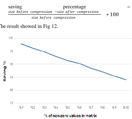
5. The saving percent according to the following relation measured.

saving percentage =

𝑠𝑖𝑧𝑒 𝑏𝑒𝑓𝑜𝑟𝑒 𝑐𝑜𝑚𝑝𝑟𝑒𝑠𝑠𝑖𝑜𝑛 −𝑠𝑖𝑧𝑒 𝑎𝑓𝑡𝑒𝑟 𝑐𝑜𝑚𝑝𝑟𝑒𝑠𝑠𝑖𝑜𝑛

𝑠𝑖𝑧𝑒 𝑏𝑒𝑓𝑜𝑟𝑒 𝑐𝑜𝑚𝑝𝑟𝑒𝑠𝑠𝑖𝑜𝑛 ∗ 100

The result showed in Fig 12.

Fig 12: saving percent according to the percent of non-zero values in matrix.

6. Figure 13 showed that the compression ratio for different matrix size almost constant for specific percent of non-zero values fixed.

Fig 13: compression ratio for different matrix size and different percent of non-zero values.

5.

DISCUSSION

The proposed algorithm compared with many other algorithms (all with 10% non-zero value). The compression ratio was about 50% ± 5% for algorithms:

Compressed Row Storage (CRS) [6], Compressed Column Storage (CCS), Modified Compressed Sparse Row (MCSR), Modified Compressed Sparse Column (MCSC), Block Compressed Row Storage (BCRS). That mean saving memory about 50% of matrix size [7] [4].

While in the proposed case the worst compression ratio was more than 15%. That means its saving memory up to 85% of matrix size.

The time needed for execute the proposed algorithm was very short as showed in figure 8, and this is very short if it is compared with other algorithms. CSC/CSR needed about 4 sec to execute matrix with size about 500 and 10% of non-zero values in matrix [4].

The compression ratio almost constant for all matrices with different sizes when the percent of zero values is fixed as showed in Fig 13.

Saving of memory storage space increased when the percent of zero values decreases.

6.

CONCLUSIONS

This paper presented a solution to the sparse matrix storage problem, using suggested algorithm based on quadtree, the alternative suggested storage format requires less storage space than all other formats.

The suggested algorithm gives less storage volume, high speed, easy to implement, easy of transpose matrix calculation.

Current algorithm checked the compression ratio, compression factor, execution time, saving percent for different matrices sizes and for different number of non-zero values in each matrix and the results was highly promised.

Its note that the compression ratio was fixed when the matrix size varied for fixed percent of non-zero values in matrix.

Results showed that storage compaction in this new method is better than other methods.

7.

REFRENCES

[1] Ivan P. Stanimirovic´ and Milan B. Tasic´, 2009. "Performance Comparison of Storage Formats for Sparse Matrices", FACTA UNIVERSITATIS (NIˇS) Ser. Math. Inform. 24 (2009), 39–51.

[2] Yousef Saad, "Iterative Methods for Sparse Linear Systems", 2003, 2nd edition, Siam publication, pp. 73-101, doi: 10.1137/1.9780898718003.ch3.

[3] Pinaki Mazumder, 1987. "Planar Decomposition for Quadtree Data Structure", Ccomputer Vision, Graphics, and Image Processing, Volume 38, Issue 3, June 1987, Pages 258–274, DOI: 10.1016/0734-189X (87)90113-7.

[5] Mats Aspn¨as, Artur Signell, and Jan Westerholm, 2007. "Efficient Assembly of Sparse Matrices Using Hashing", B. K˚agstro¨m et al. (Eds.): PARA 2006, LNCS 4699, pp. 900–907, 2007. Springer-Verlag Berlin Heidelberg 2007

[6] Tomáš Oberhuber, Atsushi Suzuki, Jan Vacata, 2011, "New Row Grouped CSR Format for Storing Sparse Matrices on GPU with Implementation in CUDA", Acta Technica journal, 56, pp 447–466.

[7] Aiyoub Farzaneh, Hossein Kheiri, and Mehdi Abbaspour Shahmersi, 2009. "An Efficient Storage Formation for Large Sparse Matrices", Commun. Fac. Sci. Univ. Ank. Series A1 Volume 58, Number 2, Pages 110 (2009) ISSN 13035991.