Chebyshev Polynomials for Solving a Class of Singular Integral Equations

(1)

http://dx.doi.org/10.4236/am.2014.54072

Chebyshev Polynomials for Solving a Class

of Singular Integral Equations

Samah M. Dardery

1

_{, Mohamed M. Allan}

2

1_{Department of Mathematics, Faculty of Science, Zagazig University, Zagazig, Egypt}

2_{Department of Mathematics, Faculty of Science and Arts Al-Mithnab, Qassim University, Qassim, KSA}

Email: [email protected], [email protected]

Received 18 November 2013; revised 18 December 2013; accepted 26 December 2013

This work is licensed under the Creative Commons Attribution International License (CC BY).

http://creativecommons.org/licenses/by/4.0/

Abstract

This paper is devoted to studying the approximate solution of singular integral equations by means of Chebyshev polynomials. Some examples are presented to illustrate the method.

Keywords

Singular Integral Equations; Cauchy Kernel; Chebyshev Polynomials; Weight Functions

1. Introduction

During the last three decades, the singular integral equation methods with applications to several basic fields of engineering mechanics, like elasticity, plasticity, aerodynamics and fracture mechanics have been studied and improved by several scientists (see [1]-[6]). Hence, it is interesting to solve numerically this type of integral eq-uations (see [7] [8]). Chebyshev polynomials are of great importance in many areas of mathematics particularly approximation theory (see [9] [10]).

In this paper we analyze the numerical solution of singular integral equations by using Chebyshev polyno-mials of first, second, third and fourth kind to obtain systems of linear algebraic equations, these systems are solved numerically. The methodology of the present work expected to be useful for solving singular integral equations of the first kind, involving partly singular and partly regular kernels. The singularity is assumed to be of the Cauchy type. The method is illustrated by considering some examples.

Singular integral equation of first kind, with a Cauchy type singular kernel, over a finite interval can be represented by

( ) ( )

_{( ) ( )}

_{( )}

1 1

,

d , d , 1 1

k t x t

t L t x t t f x x

t x

ϕ

− −

+ = − < <

−

(2)

where k t x

( ) ( )

, ,L t x, and f x

( )

are given real-valued continuous functions belonging to the class Holder of continues functions and k t t

( )

, ≠0. In Equation (1.1) the singular kernel is interpreted as Cauchy principle val-ue. Integral equation of form (1.1) and other different forms have many applications (see [1] [2] [6] [11] [12]). The theory of this equation is well known and it is presented in [13] [14]. An approximate method for solving (1.1) using a polynomial approximation of degree n has been proposed in [7].

It is well known that the analytical solutions of the simple singular integral equation

( )

_{( )}

1

d , 1 1

t

t f x x

t x

ϕ

−

= − < <

−

∫

(1.2)

at k t x

( )

, =1 and L t x

( )

, =0, for the following four cases: 1) The solution is unbounded at both end-points x= ±1, 2) The solution is bounded at both end-points x= ±1,

3) The solution is bounded at end x= −1, but unbounded at end x= +1, 4) The solution is unbounded at end x= −1, but bounded at end x= +1,

are given by [15]. In this paper the used approximate method for solving Equation (1.1) stems from recent work [10] wherein an approximate method has been developed to solve the simple Equation (1.2). The approximate method developed below appears to be quite appropriate for solving the most general type Equation (1.1). Some examples are presented to illustrate the method.

2. The

Approximate Solution

In this section we present the method of the approximate solution of Equation (1.1) in four cases. Let the unknown function

ϕ

in Equation (1.1) be approximated by the polynomial function

( )

_{( )}

( ) ( )

_{( ) (}

₎

0

1, 2, 3, 4 n

j j j

n i i

i

x W x c x j

ϕ

=

∑

Ψ ， = (2.1)

where

c

i( )j

,

i

=

0,1, 2,



,

n

are unknown coefficients, to be determined, and in case (I):

( )1

_{( )}

i x T xi

Ψ = , in case

(II): Ψ( )_i2

( )

x =U_i

( )

x , in case (III): Ψ_i( )3

( )

x =V x_i

( )

and in case (VI): Ψ_i( )4

( )

x =W x_i

( )

, where T_i, U_i, V_i

and W ii, =0,1,, ,n are The Chebyshev polynomials of the first, second, third and fourth kinds respectively can be defined by the recurrence relations [9] [16].

( )

0 1

1 2

1,

2 , 2

n n n

T x T x x

T x xT₋ x T₋ x n

= = _



= − _{≥ } (2.2)

( )

0 1

1 2

1, 2

2 , 2

n n n

U x U x x

U x xU ₋ x U ₋ x n

= = _



= − _{≥ } (2.3)

( )

0 1

1 2

1, 2 1

2 , 2

n n n

V x V x x

V x xV₋ x V₋ x n

= = − _



= − _{≥ } (2.4)

( )

0 1

1 2

1, 2 1

2 , 2

n n n

W x W x x

W x xW₋ x W₋ x n

= = + _



= − _{≥ } (2.5)

and W ii, =0,1,, ,n are the corresponding weight functions.

Substituting the approximate solution (2.1) for the unknown function into (1.1) yields

( ) 1

( )

1

_{( )}

( )

_{( )}

( )

_{( )}

0 1 1

,

d , d , 1 1

j j

n

j i j j

i i

i

k t x W t t

c t L t x W t t t f x x

t x

= − −

 _Ψ 

+ Ψ = − < <

 

−

 

 

∑

∫

(2.6)

In above Equation (2.6), we next use the following Chebyshev approximation to the kernels k t x

( )

, and

( )

,

(3)

( )

0 0

, , ,

m s

p q

k t x k x t L t x L x t

= =

≅

∑

≅

∑

(2.7)

with known expressions for K_p

( )

x and L_q

( )

x . Then (2.6) gives

( ) ( )

_{( )}

₍

₎

0

, 1 1, 1, 2, 3, 4 n

j j i i i

c

α

x f x x j

=

= − < < =

∑

(2.8)

where

( )

_{( )}

( )

_{( )}

( )

, ,

0 0

( )

m s

j j j

i p p i q q i

p q

x k x u x L x

α γ

= =

=

∑

+

∑

(2.9)

with

( )

_{( )}

1 ( )

( )

₍

₎

,

1

d , 1 1, 1, 2, 3, 4

j j

p

j i

p i

t W t t

u x t x j

t x

−

Ψ

= − < < =

−

∫

(2.10)

and

( ) 1 ( )

_{( )}

( )

_{( )}

, 1

d

j q j j

q i t W t i t t

γ

−

=

_∫

Ψ (2.11)

Let

x

_k( )j

,

j

=

1, 2,3, 4

, be the zeros of Un

( )

x T, n+₂

( )

x W, n+₁

( )

x and Vn+1

( )

x , respectively. Substituting the collocation points

x

( )_kj

,

j

=

1, 2,3, 4

into (2.8) we obtain the following systems of linear equations:

( ) ( )

( )

₍

_{) (}

₎

0

, 1, 2, , 1 , 1, 2, 3, 4 n

j j j j

i i k k

i

c

α

x f x k n j

=

= = + =

∑

 (2.12)

where

( )

( ) ( )

( )

( ) ( )

₍

_{) (}

₎

, ,

0 0

, 1, 2, , 1 , 1, 2, 3, 4

m s

j j j j j j j

i k p k p i k q k q i

p q

x k x u x L x k n j

α γ

= =

=

∑

+

∑

= _ + = (2.13)

Solving the system of Equation (2.12) for the unknown coefficients

c

i( )j

,

j

=

1, 2,3, 4

, and substituting the

values of

c

_i( )j into (2.1) we obtain the approximate solutions of Equation (1.1).

3. Numerical Examples

In this section, we consider some problems to illustrate the above method. All results were computed using FORTRAN code.

Example 1 Consider the following singular integral equation

(

2

)

( )

₍

₎

_{( )}

1 1

2 3 4 2

1 1

3

d 2 2 , 1 1

8

x t t

x t t t x x x

t x

ϕ

− −

+

+ + = − − − < <

−

∫

(3.1.1)

where

( )

2

( )

2 3

( )

4 2 3

, , , , 2 2

8

k x t = +x t L x t =x +t f t = x − x − . So, one gets

( )

(

)

0 , 1 0, 2 1, p 0, 2

k x =x k x = k x = k x = p>

( )

2

( )

(

)

0

,

1

0,

2

0,

3

1,

q

0,

3 L x

=

x L x

=

L x

=

L x

=

L x

=

q

>

Hence we find that relation (2.8) produces

( ) ( )

_{( )}

4 2

₍

₎

0

3

2 2 , 1 1, 1, 2, 3, 4 8

n j j i i i

c

α

x x x x j

=

= − − − < < =

∑

Thus (2.9) gives

( )

_{( )}

( )

_{( )}

( )

_{( )}

2 ( ) ( )

₍

_{) (}

₎

0, 2, 0, 3, , 1, 2, 3, 4 , 0,1, 2,

j j j j j

i x xu i x u i x x i i j i

(4)

Firstly, let us consider in detail the case (I),

j

=

1

, for n=3. This results in

( )1

_{( )}

1

( )

( )1

_{( )}

1 2

( )

0,. ₂ 2,. ₂

1 1

d , d , 1 1,

1 1

i i

T t t T t

u x t u x t t

t t x t t x

− −

= = − < <

− − − −

∫

(3.1.2)

( )1 1

( )

( )1 1 3

( )

0, 3,

2 2

1 1

d , d ,

1 1

i i

T t t T t

t t

γ γ

− −

= =

− −

∫

(3.1.3)

By applying the following relations

( )

(

)

( )

(

)

1 1

1

2 2

1 1

1

d π , d 0

1 1

i

T t

t U x t

t t x − t t x

− −

= =

− − − −

∫

(3.1.4)

( ) ( )

1

2 1

0

d π 0

1 _{π 2 0}

i j

i j T t T t

t i j

t _i _j

−

≠ 



=_ = =

− _ _{= ≠}

∫

(3.1.5)

It is easy to estimate the values u_0,( )1i,u( )_2,1i,

γ

_0,( )1i and

( )1 3,i

γ

. From (2.2) and (3.1.2)-(3.1.5) we get

( )

_{( )}

(

)

(

)

2

1

3 2

4 3 2

π ; 0

7

π ; 1

8

π 2 2 ; 2

1

π 4 4 ; 3

8 i

x x i

x

x x i

x x x x i

α

 + =



  _{+ +}  ₌

  

  

= 

+ =

 

 

 ₊ ₋ _{− +} ₌

 

  



(3.1.6)

By choosing the collocation points

(

)

(

) (

)

2 1 π

cos , 1, 2, 3, 4

2 2

k

x k

n

 − 

= _ _ =

+

  , for n=3, we obtain the following system of linear equations:

( ) ( )

_{( )}

3 1 1 0

, 1, 2, 3, 4

i i k k

i

c

α

x f x k

=

= =

∑

By solving this system for the unknown coefficients

c

_i( )1

,

i

=

0,1, 2,3

that produces

( ) ( )

1 1

0 1

1 1

2 3

0.3183098, 0.1591549

c c



= = − _



= − = _ (3.1.7)

From (3.1.7) we obtain the approximate solution of Equation (3.1.1) in the form

( )

(

3 2

)

2

1 π 1

n x x x x

x

ϕ ≅ − − +

− (3.1.8)

Which coincides with the exact solution. The error of approximate solution (3.1.8) of Equation (3.1.1) at 20

n= is given by Table 1.

Secondly, let us consider in detail the case (II),

j

=

2

( )2

_{( )}

1 2

( )

( )2

_{( )}

1 2 2

( )

0,. 2,.

1 1

d , d , 1 1,

i i

t U t t t U t

u x t u x t t

t x t x

− −

= = − < <

− −

∫

(3.1.9)

( )2 1 2

_{( )}

( )2 1 2 3

_{( )}

0, 3,

1 1

1 d , 1 d ,

i t U ti t i t t U ti t

γ γ

− −

=

_∫

− =

_∫

− (3.1.10)

(5)

( )

_{( )}

2 1 1 1 1 d π i i

t U t

t T x

t x +

−

= − −

∫

(3.1.11)

( ) ( )

1

2

1

0

1 d _π

2

i j

i j t U t U t t

i j − ≠   − _{= } = 

∫

(3.1.12)

It is easy to estimate the values u0,( )2i,u2,( )2i,

γ

0,( )2i and

( )2 3,i

γ

. From the relations (2.3) and (3.1.9)-(3.1.12) we get

( )

_{( )}

(

3 2

)

4 3 2

2

5 4 3 2

6 5 4 3 2

π ₂ ₀

2

3

π 2 2 1

8 1

π 4 4 3 3 2

4 1

π 8 8 8 8 3

16 i

x x x i

x x x x i

x

x x x x x i

x x x x x x i

α − + − =     − _ + − − − _ =  _ _  =  _ _ − _ + − − + _ =  _ _    − _ + − − + + − _ =  _ _  (3.1.13)

By choosing the collocation points ( )

(

)

(

) (

)

2 2 1 π

cos , 1, 2, 3, 4

2 2 k k x k n  −  = _ _ = +

  , for n=3,we obtain the following system of linear equations :

( ) ( )

( )

3

2 2 2 2

0

, 1, 2, 3, 4

i i k k

i

c

α

x f x k

=

= =

∑

c

_i( )2

,

i

=

0,1, 2,3

that produces

( ) ( )

2 2

0 1

2 8 2 9

2 3

0.6366197, 0.3183099

2.279989 10 , 7.819254 10

c c

c − c −



= = − _



= × = − × _ (3.1.14)

From (3.1.14) we obtain the approximate solution of Equation (3.1.1) in the form

( )

2 1 2

(

)

1 π n

x

x x

ϕ ≅ − − (3.1.15)

Which coincides with the exact solution. The error of approximate solution (3.1.15) of Equation (3.1.1) at 20

Thirdly, let us consider in detail the case (III),

j

=

3

( )3

_{( )}

1

( )

( )3

_{( )}

1 2

( )

0,. 2,.

1 1

d , d , 1 1,

1 1

i i

V t t V t

t t

u x t u x t t

t t x t t x

− −

+ +

= = − < <

− − − −

∫

(3.1.16)

( )3 1

_{( )}

( )3 1 3

_{( )}

0, 3,

1 1

d , d ,

1 1

i i i i

t t

V t t t V t t

t t γ γ − − + + = = − −

∫

(3.1.17)

By applying the following relations

( ) ( )

1 1 0 1 d π

1 i j

i j t

V t V t t

i j t − ≠  + =  ₌ − _

∫

(3.1.18)

( )

_{( )}

1 1 1 d π 1 i i V t t

t W x

t t x −

+ ₌

− −

∫

(3.1.19)

It is easy to estimate the values u_0,( )3i,u_2,( )3i,

γ

_0,( )3i and

(6)

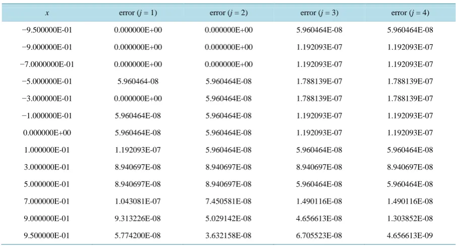
[image:6.595.86.539.98.342.2]

Table 1. Illustrates errors of approximate solutions of Equation (3.1.1) in Cases (I)-(IV) at n = 20.

x error (j = 1) error (j = 2) error (j = 3) error (j = 4) −9.500000E-01 0.000000E+00 0.000000E+00 5.960464E-08 5.960464E-08 −9.000000E-01 0.000000E+00 0.000000E+00 1.192093E-07 1.192093E-07 −7.0000000E-01 0.000000E+00 0.000000E+00 1.192093E-07 1.192093E-07 −5.000000E-01 5.960464-08 5.960464E-08 1.788139E-07 1.788139E-07 −3.000000E-01 0.000000E+00 5.960464E-08 1.788139E-07 1.788139E-07 −1.000000E-01 5.960464E-08 5.960464E-08 1.192093E-07 1.192093E-07

0.000000E+00 5.960464E-08 5.960464E-08 1.192093E-07 1.192093E-07 1.000000E-01 1.192093E-07 5.960464E-08 5.960464E-08 5.960464E-08 3.000000E-01 8.940697E-08 8.940697E-08 8.940697E-08 8.940697E-08 5.000000E-01 8.940697E-08 8.940697E-08 5.960464E-08 5.960464E-08 7.000000E-01 1.043081E-07 7.450581E-08 1.490116E-08 1.490116E-08 9.000000E-01 9.313226E-08 5.029142E-08 4.656613E-08 1.303852E-08 9.500000E-01 5.774200E-08 3.632158E-08 6.705523E-08 4.656613E-09

From the relations (2.4) and (3.1.16)-(3.1.19) we get

( )

_{( )}

2

3 2

3

4 3 2

5 4 2

7

π 2 2 0

8 7

π 2 3 1

8 1

π 4 6 2

8 1

π 8 12 5 3

8 i

x x i

x x x i

t

x x x x i

α

  ₊ ₊  ₌

 

  



  ₊ _{+ +}  ₌

  

  

= 

 

 ₊ ₊ _{− +} ₌

 

  



 

 ₊ ₋ _{+ +} ₌

 

  



(3.1.20)

(

) (

)

3 2 π

cos , 1, 2, 3, 4

2 3

k

x k

n

 

= _ _ =

+

  , for n=3, we obtain the following system of linear equations :

( ) ( )

( )

3

3 3 3 3

0

, 1, 2, 3, 4

i i k k

i

c

α

x f x k

=

= =

∑

c

_i( )3

,

i

=

0,1, 2,3

that produces

( ) ( )

3 3

0 1

3 3 8

2 3

0.3183098, 0.4774647,

0.1591549, 1.330901 10

c c

c c −



= = − _



= = × _ (3.1.21)

From (3.1.21) we obtain the approximate solution of Equation (3.1.1) in the form of

( )

2 1

(

2

)

2 1

π 1 n

x

x x x

x

ϕ ≅ + − +

− (3.1.22) Which coincides with the exact solution. The error of approximate solution (3.1.22) of Equation (3.1.1) at

20

(7)

( )4

_{( )}

1

( )

( )4

_{( )}

1 2

( )

0,. 2,.

1 1

d , d , 1 1,

1 1

i i

W t t W t

t t

u x t u x t t

t t x t t x

− −

= = − < <

+ − + −

∫

(3.1.23)

( )4 1

_{( )}

( )4 1 3

_{( )}

0, 3,

1 1

d , d ,

1 1

i i i i

t t

W t t t W t t

t t

γ γ

− −

= =

+ +

∫

(3.1.24)

By applying the relations

( ) ( )

1

0 1

d π

1 i j

i j t

W t W t t

i j t

−

≠  −

=  ₌

+ _

∫

(3.1.25)

( )

_{( )}

1

1 1

d π

1 i

i W t

t

t V x

t t x −

− _{= −}

+ −

∫

(3.1.26)

It is easy to estimate the values u_0,( )4_i,u_2,( )4_i,

γ

_0,( )4_i and

γ

_3,( )4_i . From the relations (2.5) and (3.1.23)-(3.1.26) we get

( )

_{( )}

3 2

4

4 3 2

5 4 3 2

7π

; 0

8

7

π 2 ; 1

8 1

π 4 2 3 ; 2

8 1

π 8 4 8 3 ; 3

8 i

i

x x x i

x

x x x x i

x x x x x i

α

−

 ₌

 

 

− _ + − − _ =

 _ _



=  _ _

− _ + − − + _ =

  



 

− _ + − − + − _ =

 _ _



(3.1.27)

(

)

(

) (

)

4 2 1 π

cos , 1, 2, 3, 4

2 3

k

x k

n

 − 

= _ _ =

+

( ) ( )

( )

3

4 4 4 4

0

, 1, 2, 3, 4

i i k k

i

c

α

x f x k

=

= =

∑

c

_i( )4

,

i

=

0,1, 2,3

that produces

( ) ( )

4 4

0 1

4 4 8

2 3

0.3183098, 0.1591549

0.1591549, 2.358931 10

c c

c c −



= = _



= − = × _ (3.1.28)

( )

2 1

(

2

)

1 π 1

n

x

x x

x

ϕ ≅ − − −

+ (3.1.29)

which coincides with the exact solution. The error of approximate solution (3.2.29) of Equation (3.2.1) at 20

Example 2. Consider the following singular integral equation

( )

₍

₎

_{( )}

1 1

3 2 3

1 1

d d

t

t x xt t t x x

t x

ϕ

− −

+ + = +

−

∫

(3.2.1)

which corresponds with k t x

( )

, =1 and

L t x

( )

,

=

x

3

+

xt

2. So one gets

( )

(

)

0 1, p 0, 0

k x = k x = p>

( )

3

( )

( ) (

)

0

,

1

0,

2

,

q

0

2

(8)

Hence we find that relation (2.8) produces

( ) ( )

_{( )}

3

₍

₎

0

, 1 1, 1, 2, 3, 4 n

j j i i i

c

α

x x x x j

=

= + − < < =

∑

Thus (2.9) gives

( )

_{( )}

( )

_{( )}

3 ( ) ( )

₍

_{) (}

₎

0, 0, 2, , 1, 2, 3, 4 , 0,1, 2,

j j j j

i x u i x x i x i j i

α

= +

γ

+

γ

= = _

Firstly, let us consider in detail the case (I),

j

=

1

, for n=3. This results in ( )1 1 2

( )

2,

2 1

d , 1

i i

t T t t t

γ

−

= −

∫

(3.2.2)

From the relations (3.1.2)-(3.1.5) and (3.2.2) we obtain

( )

_{( )}

(

)

(

)

3

1

2

π 2 0

π 1

9π 4 2

π 4 1 3

i

x x i

i x

x i

α

 + =



 =

=  ₌



 ₋ ₌



(3.2.3)

By choosing the collocation points

(

)

(

) (

)

2 1 π

cos , 1, 2, 3, 4

2 2

k

x k

n

 − 

= _ _ =

+

( ) ( )

_{( )}

3 1 1 0

, 1, 2, 3, 4

i i k k

i

c

α

x f x k

=

= =

∑

c

_i( )1

,

i

=

0,1, 2,3

that produces

( ) ( )

1 1 8

0 1

1 1 8

2 3

0.3183098, 1.090772 10

0.07073557, 1.830649 10

c c

−



= = × _



= = × _ (3.2.4)

( )

(

2

)

2

1

7 4 9π 1

n x x

x

ϕ ≅ +

− (3.2.5)

which coincides with the exact solution. The error of approximate solution (3.2.5) of equation (3.2.1) at n=20 is given by Table 2.

Secondly, let us consider in detail the case (II),

j

=

2

( )2 1 2 2

_{( )}

2, 1

1 d ,

i t t U ti t

γ

−

=

_∫

− (3.2.6)

By applying the relations (3.1.9)-(3.1.12) and (3.2.6) we get

( )

_{( )}

(

)

(

)

3

2 2

3

4 2

π 7

0

2 4

π 2 1 1

25

π 4 2

8

π 8 8 1 3

i

x

x i

x

x i

x x i

α

  ₋  ₌

 

  



− − =

 = 

 

− _ − _ =

 _ _



− − + =



(3.2.7)

(

)

(

) (

)

2 2 1 π

cos , 1, 2, 3, 4

2 2

k

x k

n

 − 

= _ _ =

+

(9)

[image:9.595.87.538.108.351.2]

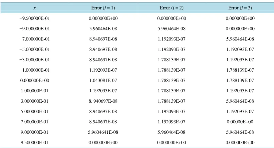
Table 2. Illustrates errors of approximate solutions of Equation (3.2.1) in Case (I), Case (II) and Case (IV) respectively at n

= 20.

x Error (j = 1) Error (j = 2) Error (j = 3)

−9.500000E-01 0.000000E+00 0.000000E+00 0.000000E+00

−9.000000E-01 5.960464E-08 5.960464E-08 0.000000E+00

−7.000000E-01 8.940697E-08 1.192093E-07 5.960464E-08

−5.000000E-01 8.940697E-08 1.192093E-07 1.192093E-07

−3.000000E-01 8.940697E-08 1.788139E-07 1.192093E-07

−1.000000E-01 1.192093E-07 1.788139E-07 1.788139E-07

0.000000E+00 1.043081E-07 1.788139E-07 1.788139E-07

1.000000E-01 1.192093E-07 1.788139E-07 1.192093E-07

3.000000E-01 8. 940697E-08 1.788139E-07 5.960464E-08

5.000000E-01 8.940697E-08 1.192093E-07 1.192093E-07

7.000000E-01 8.940697E-08 1.192093E-07 0.00000E+00

9.000000E-01 5.9604641E-08 5.960464E-08 5.960464E-08

9.500000E-01 0.000000E+00 0.000000E+00 0.000000E+00

system of linear equations:

( ) ( )

( )

3

2 2 2 2

0

, 1, 2, 3, 4

i i k k

i

c

α

x f x k

=

= =

∑

c

i( )2

,

i

=

0,1, 2,3

that produces

( ) ( )

2 2 9

0 1

2 2 8

2 3

1.170559, 1.331665 10

0.2258973, 1.644008 10

c c

−



= − = − × _



= − = − × _ (3.2.8)

( )

1 2 2

92 88 31π

n

x

x x

ϕ ≅− − _ + _ (3.2.9)

which coincides with the exact solution. The error of approximate solution (3.2.9) of Equation (3.2.1) at n=20 is given by Table 2.

Thirdly, In case (IV),

j

=

4

( )4 1 2

_{( )}

2, 1

1

d , 1

i i

t

t W t t t

γ

− − =

+

∫

(3.2.10)

By applying the relations (3.1.23)-(3.1.26) and (3.2.10) we get

( )

_{( )}

(

)

3

4

2

3 2

π 1 0

2 9

π 1 1

4 9

π 4 1 2

4

π 8 4 4 1 3

i

x

x i

x

x i

x x x i

α

  _{+ −}  ₌

 

  



 _ _

− − =

  

 _ _

= 

 _ _

− − − =

 _ _



− − − + =



(10)

(

)

(

) (

)

4 2 1 π

cos , 1, 2, 3, 4

2 3

k

x k

n

 − 

= _ _ =

+

  , for n=3, we obtain the following system of linear equations:

( ) ( )

( )

3

4 4 4 4

0

, 1, 2, 3, 4

i i k k

i

c

α

x f x k

=

= =

∑

c

_i( )4

,

i

=

0,1, 2,3

that produces

( )4 ( )4 ( )4 ( )4

0 1

0.5852794,

2 3

0.1129487

c

=

c

= −

c

=

c

= −

(3.2.12)

( )

1 1

(

₁

)

(

_{92 88} 2

)

31π 1 n

x

x x x

x

ϕ ≅ − − + +

+ (3.2.13)

which coincides with the exact solution. The error of approximate solution (3.2.13) of Equation (3.2.1) at 20

Similarly, doing the same operations as we did for Case (I), Case (II) and Case (IV), one can solve for Case (III) .

Example 3. Consider the following singular integral equation

( )

₍

₎

_{( )}

1 1

2 2 2

1 1

3

d d 2

2

t

t x t t t x x

t x

ϕ

− −

−

+ + = +

−

∫

, (3.3.1)

which corresponds with k t x

( )

, =1 and

L t x

( )

,

=

x

2

+

t

2. So, one gets

( )

(

)

0 1, p 0, 0

k x = k x = p>

( )

2

( )

( ) (

)

0

,

1

0,

2

1,

q

0

2 L x

=

x L x

=

L x

=

L x

=

q

>

Hence the relation (2.8) produces

( ) ( )

_{( )}

2

0

3

2 , 1 1, 1, 2, 3, 4 2

n j j i i i

c

α

x x x x j

=

−

= + − < < =

∑

(3.3.2)

where (2.9) gives

( )

_{( )}

( )

_{( )}

2 ( ) ( )

₍

_{) (}

₎

0, 0, 2, , 1, 2, 3, 4 , 0,1, 2,

j j j j

i x u i x x i i j i

α

= +

γ

+

γ

= = 

Firstly, let us consider in detail the case (II),

j

=

2

, for n=3. From (3.1.9)-(3.1.12) and (3.2.6) we get

( )

_{( )}

(

)

(

)

(

)

(

)

2

2 2

3

4 2

π

4 8 1 0

8

π 2 1 1

π

32 24 1 2

8

π 8 8 1 3

i

x x i

x i

x

x x i

α

 ₋ ₊ ₌

 

− − =



= ₋

 ₋ ₋ ₌

 

− − + =



(3.3.3)

By solving the system (3.3.2), at the collocation points ( )

(

)

(

) (

)

2 2 1 π

cos , 1, 2, 3, 4

2 2

k

x k

n

 − 

= _ _ =

+

  , for the unknown

coefficients

c

i( )2

,

i

=

0,1, 2,3

we obtain

( ) ( )

2 2

0 1

2 8 2 8

2 3

0.6366197, 0.07957754

1.746461 10 , 1.827517 10

c c

c − c −



= − = _



= × = × _ (3.3.4)

So the approximate solution of Equation (3.3.1) is given by

( )

1 2

(

)

4 2π n

x

x x

(11)

which coincides with the exact solution, the error of the approximate solution (3.3.5) of Equation (3.3.1) at 20

Secondly, in case (III),

j

=

3

( )3 1 2

_{( )}

2, 1

1

d , 1

i i

t

t V t t t

γ

− + =

−

∫

(3.3.6)

From (3.1.16)-(3.1.19) and (3.3.6) we get

( )

_{( )}

(

)

2

3

2

3 2

3

π 0

2 5

π 2 1

4 3

π 4 2 2

4

π 8 4 4 1 3

i

x i

x

x x i

x x x i

α

  ₊  ₌

 

  



  ₊  ₌

  

  

= 

  ₊ ₋  ₌

 _ _



 ₊ ₋ ₊ ₌



(3.3.7)

By solving the system (3.3.2), at the collocation points ( )

(

) (

)

3 2 π

cos , 1, 2, 3, 4

2 3

k

x k

n

 

= _ ₊ _ =

  , for the unknown

coefficients

c

_i( )3

,

i

=

0,1, 2,3

we obtain

( ) ( )

3 3

0 1

3 3 9

2 3

0.3183099, 0.3580987,

0.03978872, 8.155105 10

c c

c c −



= − = _



= − = − × _ (3.3.8)

Hence, the approximate solution of Equation (3.3.1) is given by

( )

1 1

(

2

)

5 4

2π 1 n

x

x x x

x

ϕ ≅ − + − +

− (3.3.9) which coincides with the exact solution, the error of the approximate solution (3.3.9) of Equation (3.3.1) at

20

[image:11.595.97.542.107.440.2] [image:11.595.89.537.486.720.2]

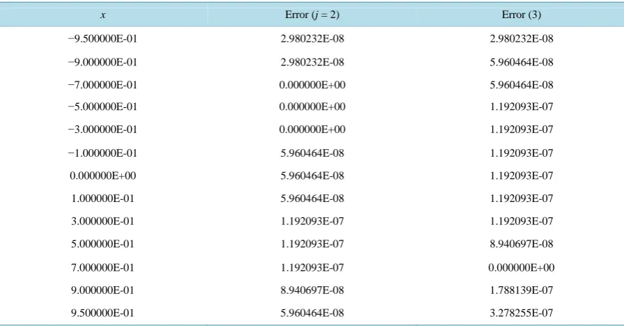
Table 3. Illustrates errors of approximate solutions of Equation (3.3.1) in Case (II) and Case (III) at n = 20.

x Error (j = 2) Error (3)

−9.500000E-01 2.980232E-08 2.980232E-08

−9.000000E-01 2.980232E-08 5.960464E-08

−7.000000E-01 0.000000E+00 5.960464E-08

−5.000000E-01 0.000000E+00 1.192093E-07

−3.000000E-01 0.000000E+00 1.192093E-07

−1.000000E-01 5.960464E-08 1.192093E-07

0.000000E+00 5.960464E-08 1.192093E-07

1.000000E-01 5.960464E-08 1.192093E-07

3.000000E-01 1.192093E-07 1.192093E-07

5.000000E-01 1.192093E-07 8.940697E-08

7.000000E-01 1.192093E-07 0.000000E+00

9.000000E-01 8.940697E-08 1.788139E-07

(12)

Similarly, doing the same operations as we did for Case (II) and Case (III), one can solve for Case (I) and Case (IV).

4. Conclusion

Numerical results (Tables 1-3) show that the errors of approximate solutions of Examples 1-3 in different Cases with small value of n are very small. These show that the methods developed are very accurate and in fact for a linear function give the exact solution.

References

[1] Chakrabarti, A. (1989) Solution of Two Singular Integral Equations Arising in Water Wave Problems. ZAMM, 69, 457-459. http://dx.doi.org/10.1002/zamm.19890691209

[2] Ladopoulous, E.G. (2000) Singular Integral Equations Linear and Non-Linear Theory and Its Applications in Science and Engineering. Springer, Berlin.

[3] Ladopoulous, E.G. (1987) On the Solution of the Two-Dimensional Problem of a Plane Crack of Arbitrary Shape in an Anisotropic Material. Engineering Fracture Mechanics, 28, 187-195. http://dx.doi.org/10.1016/0013-7944(87)90212-8

[4] Zabreyko, P.P. (1975) Integral Equations—A Reference Text. Noordhoff, Leyden. http://dx.doi.org/10.1007/978-94-010-1909-5

[5] Prossdorf, S. (1977) On Approximate Methods for the Solution of One-Dimensional Singular Integral Equations. Ap-plicable Analysis, 7, 259-270.

[6] Zisis, V.A. and Ladopoulos, E.G. (1989) Singular Integral Approximations in Hilbert Spaces for Elastic Stress Analy-sis in a Circular Ring with Curvilinear Cracks. Indus. Math., 39, 113-134.

[7] Chakrabarti, A. and Berghe, V.G. (2004) Approximate Solution of Singular Integral Equations. Applied Mathematics Letters, 17, 553-559. http://dx.doi.org/10.1016/S0893-9659(04)90125-5

[8] Abdou, M.A. and Naser, A.A. (2003) On the Numerical Treatment of the Singular Integral Equation of the Second Kind. Applied Mathematics and Computation, 146, 373-380. http://dx.doi.org/10.1016/S0096-3003(02)00587-8

[9] Abdulkawi, M., Eshkuvatov, Z.K. and Nik Long, N.M.A. (2009) A Note on the Numerical Solution of Singular Integral Equations of Cauchy Type. International Journal of Applied Mathematics and Computer Science, 5, 90-93.

[10] Eshkuvatov, Z.K., Nik Long, N.M.A. and Abdulkawi, M. (2009) Approximate Solution of Singular Integral Equations of the First Kind with Cauchy Kernel. Applied Mathematics Letters, 22, 651-657.

http://dx.doi.org/10.1016/j.aml.2008.08.001

[11] Gakhov, F.D. (1966) Boundary Value Problems. Addison-Wesley, Boston.

[12] Martin, P.A. and Rizzo, F.J. (1989) On Boundary Integral Equations for Crack Problems. Proceedings of the Royal So-ciety A, 421, 341-345. http://dx.doi.org/10.1098/rspa.1989.0014

[13] Sheshko, M. (2003) Singular Integral Equations with Cauchy and Hilbert Kernels and Their Approximated Solutions. The Learned Society of the Catholic University of Lublin, Lublin. (in Russian)

[14] Muskhelishvili, N.I. (1977) Singular Integral Equations. Noordhoff International Publishing, Leyden. http://dx.doi.org/10.1007/978-94-009-9994-7

[15] Lifanov, I.K. (1996) Singular Integral Equation and Discrete Vortices. VSP, Leiden.