A MODEL FOR MEASURING ARTICLES KNOWLEDGEABILITY LEVELS

ISSN: 1992-8645 www.jatit.org E-ISSN: 1817-3195

LEAST-MEAN DIFFERENCE ROUND ROBIN (LMDRR) CPU

SCHEDULING ALGORITHM

1

D. ROHITH ROSHAN, 2DR. K. SUBBA RAO

1

M.Tech (CSE) Student, Department of Computer Science and Engineering, KL University, India.

2

Professor, Department of Computer Science and Engineering, KL University, India.

E-mail: [email protected], [email protected]

ABSTRACT

This article presents a variant of Round Robin Algorithm called Least Mean-Difference Round Robin (LMDRR) Algorithm. First, it calculates the mean of all processes burst times. Then it obtains the difference of each process burst time with the calculated mean. From those differences, it selects the least difference and assigns it to the CPU for executing it for a time slice. When the time slice is expired it suspends the process and checks the remaining burst time of the process if it is less than time quantum then it immediately executes the process, if the remaining time is greater than time quantum then it selects the process with next least difference and execute it for another time slice. This entire process will be repeated until all the processes in the ready queue are finished. The experimental results are compared with Round Robin and Mean-Difference Round Robin algorithms and found that proposed algorithm succeeded in improving CPU efficiency.

Keywords: Burst Time, Turnaround Time, Waiting Time, CPU Scheduling, Pre-emptive Scheduling, non Pre-emptive Scheduling, LMDRR.

1. INTRODUCTION

Among key resources of a computer, CPU is the most important component since it is the heart of the system. Hence, scheduling is necessary for OS (Operating System) [1]. For utilizing resources productively, they should be shared among multiple resources and users [2]. Maximum sharing of resources relies on the effective scheduling of processes in a system and its users for the processor, which makes scheduling the processes a key ingredient of multiprogramming OS. Because the processor is a key resource, process scheduling also called CPU scheduling, turns out to be a predominant aspect in accomplishing objectives mentioned above [1].

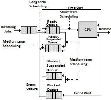
OS can constitute 3 different types of schedulers: long, medium and short-term schedulers as shown in Figure 1.

There are several scheduling algorithms available that differ in efficiency basing on environment that means we believe an algorithm is good in some cases and not in other and vice-versa. A good CPU scheduler should satisfy the following criteria:

Figure 1. Queue Diagram For Scheduling

● Maximize Throughput. (Throughput means number of jobs completed per unit of time.) ● Minimize Response Time. (Response Time is

the time taken to respond for a program.) ● Minimize Turnaround Time. (Turnaround

Time is the total time required for process from

submission to its completion.)

ISSN: 1992-8645 www.jatit.org E-ISSN: 1817-3195 ● Maximize CPU Efficiency. (Keeping CPU

busy 100% with 0% wastage of CPU cycles.) ● Assure fairness for all jobs. (Give equal

amount of CPU time for all jobs.)

To resolve this issue, the CPU Scheduler in most cases utilizes a timing mechanism and interrupts running jobs periodically for a lapse of fixed time slice. After that, the scheduler halts all activities of the job and reschedules it into ready queue. Now, the CPU is allocated another job that runs unless: the timer goes off, an I/O command is issued by the job, or the job is completed. Accordingly, the job is moved to Ready, Wait or Finished queues, respectively. This type of scheduling is called Preemptive Scheduling and the other one is Non-Preemptive Scheduling, which work without interrupts.

2. LITERATURE SURVEY

To allot the CPU with jobs in the system, the scheduler depends on Process Scheduling Algorithm which is based on a particular strategy. In early OS non-preemptive scheduling strategies were used, but, in the recent interactive systems, the algorithm should instantly respond to user requests. The scheduling algorithms that are used often were:

2.1 First Come First Serve (FCFS)

FCFS scheduling algorithm services the requests as they arrive. It is the easiest scheduling algorithm and utilized as a standard to differentiate other algorithms. FCFS is suitable in conditions in which there is only one application access the resource [3].

2.2 Shortest Job First (SJF)

SJF [4] is non-preemptive and attempts to increase the response time of tasks regarding FCFS. But it needs additional knowledge of every job's service time. It selects the job with the smallest time. The OS will suspend the current job if the next job has less burst time. The main issue with SJF is that larger processes need to wait for a long time.

2.3 Priority Based Scheduling

This algorithm allocates every process to CPU basing on the priority associated with it. The processes with higher priorities are executed first and processes with lower priorities are executed later. In the event that different processes with similar priorities, the CPU is allocated to processes on the premise of FCFS. This scheduling algorithm

can be either preemptive or non-preemptive depending on nature and environment [5].

2.4 Round Robin Scheduling (RR)

RR is the easiest among CPU scheduling algorithms in an OS, and that allots time slices to every process in circular order and in uniform segments [6] [7] [8], dealing with all process without any priority [9], possibly, the main trouble in RR is with the time slice [10] [10] [11] [12]. Jobs are arranged in the READY Queue in FCFS strategy. The scheduler chooses the first job in the queue and then sets the timer to a time slice, after that it allots the job to the CPU. If the job is finished, then all of its resources are released and removed from the queue. If the job is not finished and the timer goes off, then it is preempted and placed at the end of queue.

2.5 Mean-Difference Round Robin (MDRR)

The existing [13] system minimizes the performance characteristics such as waiting time, context switches and turn-around time by executing following steps:

Step 1: Calculate the mean of the burst time for all process.

Step 2: Compute the differences for each process burst time and the mean.

Step 3: Select the process with largest difference value and allot the CPU with the selected process for a time slice.

Step 4: Repeat 1 and 3 steps until all the jobs are finished in READY queue.

In the following section, we present our LMDRR algorithm which enhances CPU scheduling more effectively than Round Robin (RR) and Mean Difference Round Robin (MDRR).

3. METHODOLOGY

ISSN: 1992-8645 www.jatit.org E-ISSN: 1817-3195

3.1 Proposed Algorithm Input:

BT[] - Array of burst times. PID[] - Array of processes. N - Total number of processes. δ - Time Quantum.

Output:

Average waiting time (AWT) of all processes. Average turnaround time (ATT) of all processes.

Algorithm:

Step 1: Compute the mean of burst time of every process in the ready queue.

Sum =+ BT[i]; Mean=Sum/N;

Step 2: Compute the mean differences for every process in the ready queue.

D[] = Mean-BT[i];

Step 3: Identify the process with smallest difference value.

Find Smin[] and PID[];

Avail CPU for executing the process for one time slice.

PID[]. BT[i] = BT[i]-δ;

Step 4: If the remaining burst time of current running process is less than or equal to TQ (Time Quantum), then continue its execution.

PID[]. BT[i] <= δ;

Step 5: Later, completing the step 4, select the next process which is having the smallest difference value.

Find Smin-1 [] and PID[];

Execute it and repeat step 4. If any two processes have the same mean difference value, then find the shortest process and assign it to the CPU.

Step 6: For all the processes in the ready queue repeat step 5.

Step 7: Repeat step 1 through step 6 until all the processes in the ready queue are finished.

Step 8: Calculate the average waiting time of all the processes in the ready queue.

AWT=Σ Wi/N;

Step 9: Calculate the average turnaround time of all the processes in the ready queue. ATT=Σ Ti/N;

D [] – Array of Mean-Difference.

Smin – Process with smallest difference value. Smin-1 – Process with next smallest difference

value.

Wi – Waiting time of i th process. Ti – Turnaround time of i th process.

4. EXPERIMENTAL RESULTS

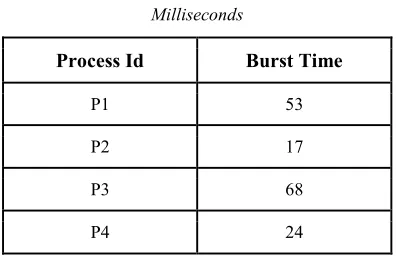
Example 1: Consider the set of processes, in the order p1, p2, p3, p4 shown in the Table 1, presumed to have arrived at time t0, with the time quantum 10, 15, 20, 25 and duration of the CPU burst times given in milliseconds.

Table 1: Processes With Their Burst Times In Milliseconds

Process Id Burst Time

P1 53

P2 17

P3 68

P4 24

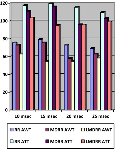
In the below Table 2 a comparative study of the efficiency of the proposed LMDRR, RR and the MDRR algorithm with different Time Quantum values is showing that the proposed LMDRR algorithm has the minimum Average Waiting Time and Average Turnaround Time.

Table 2: RR, MDRR And The Proposed LMDRR Algorithm Performance Comparison

Time Slice

10 msec

15 msec

20 msec

25 msec

RR AWT 75.5 79.25 73 69.25

MDRR AWT

73 75.5 58 63

LMDRR AWT

63 54.75 54.75 58.5

RR ATT 117.5 119.5 115.5 109.75

MDRR ATT

111 116 96 103

LMDRR ATT

103.5 95.25 95.5 99

ISSN: 1992-8645 www.jatit.org E-ISSN: 1817-3195

The mean of burst times in Table 1 is :

The mean-differences of the processes are shown in Table 3.

Table 3: Processes Burst Time And Mean-Difference

Process Burst Time Mean-Difference

P1 53 12.5

P2 17 23.5

P3 68 27.5

P4 24 16.5

Now the process with least mean difference is allotted to CPU and then the process with next least mean-difference. Like this processes are allotted to CPU in the order P1, P4, P2, P3. In this iteration P2 and P4 are completed.

After the first iteration the algorithm again calculates the mean and differences for the remaining processes

The mean-differences of the remaining processes are shown in Table 4.

Table 4: Remaining Processes Burst Time And Mean-Difference

Process Burst Time Mean-Difference

P1 28 7.5

P3 43 7.5

Since both the processes have same mean difference the algorithm selects the process in sequential order i.e., P1. As the P1 completes one time slice, it has only burst time of 3msec is remaining which is less than the time quantum 25 so immediately it will be executed. After that P3 will be allotted. Like this, the procedure repeats until all the processes are finished. The complete Gantt chart is shown in the Figure 2.

Figure 2: Gantt Chart For LMDRR Algorithm

The comparison graph of RR, MDRR and LMDRR algorithms is presented in Figure 3.

0 20 40 60 80 100 120

10 msec 15 msec 20 msec 25 msec

RR AWT MDRR AWT LMDRR AWT

RR ATT MDRR ATT LMDRR ATT

Figure 3: Performance Comparison Graph Of RR, MDRR And LMDRR

Example 2: Consider the set of processes, in the order p1, p2, p3, p4, p5 shown in the Table 5, presumed to have arrived at time t0, with the time quantum 10, 14, 16, 18 and duration of the CPU burst times given in milliseconds.

Table 5. Processes With Their Burst Times In Milliseconds

Process Id Burst Time

P1 51

P2 22

P3 42

4 18

P5 62

ISSN: 1992-8645 www.jatit.org E-ISSN: 1817-3195 Table 6: RR, MDRR And The Proposed LMDRR

Algorithm Performance Comparison

Time Slice

10 msec

14 msec

16 msec

18 msec

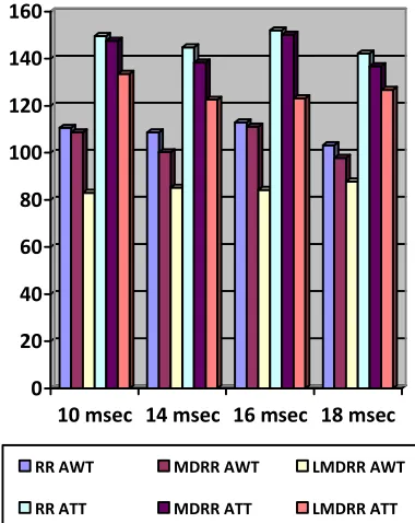
RR AWT 110.6 108.6 113 103.2

MDRR AWT

108.6 100.2 111.2 97.8

LMDRR AWT

83 85.2 84.2 87.8

RR ATT 149.6 144.8 152 142.2

MDRR ATT

147.6 138.4 150.2 136.8

LMDRR ATT

133.6 122.6 123.2 126.8

LMDRR Scheduling:

The mean of the burst times in Table 5 is:

The mean-differences of the processes are shown in Table 7.

Table 7: Processes Burst Time And Mean-Difference

Process Burst Time Mean-Difference

P1 51 12

P2 22 17

P3 42 3

P4 18 21

P5 62 23

Now the process with least mean difference is allotted to CPU and then the process with next least mean-difference. Like this processes are allotted to CPU in the order P3, P1, P2, P4, P5. In this iteration P2 and P4 are completed.

After the first iteration the algorithm again calculates the mean and differences for the remaining processes

The mean-differences of the remaining processes are shown in Table 8.

Table 8: Remaining Process Burst Times And Mean-Differences

Process Burst Time Mean-Difference

P1 33 0.66

P3 24 9.66

P5 44 10.34

The processes are allotted to CPU in the order P1, P3, P5. In this iteration process P1 and P3 will be completed. Like this, the procedure repeats until all the processes are finished. The complete Gantt chart is shown in the Figure 4.

Figure 4: Gantt Chart For LMDRR Algorithm

The comparison graph of RR, MDRR and LMDRR algorithms is presented in Figure 5.

0 20 40 60 80 100 120 140 160

10 msec 14 msec 16 msec 18 msec

RR AWT MDRR AWT LMDRR AWT

RR ATT MDRR ATT LMDRR ATT

ISSN: 1992-8645 www.jatit.org E-ISSN: 1817-3195

5. CONCLUSION

This paper presents a form of Round Robin scheduling algorithm called Least Mean-Difference Round Robin (LMDRR) algorithm. The algorithm presented in the paper computes the average on total processes burst time resided in the ready queue. Then, it ascertains the differences of calculated average and process burst times. In those differences, the algorithm takes the process with the smallest difference value and allots CPU to that process for one time slice. When the time slice is expired, the subsequent process from the ready queue is taken which is having the smallest difference value and it will be executed for another time slice. The algorithm assures the repetition of this procedure until all processes are finished in the ready queue. The algorithm’s efficiency is evaluated with two examples. Experimental results are compared with MDRR and RR algorithm and found that the proposed LMDRR algorithm exhibited better optimal scheduling.

REFRENCES:

[1] Shah, Syed Nasir Mehmood, Ahmad Kamil Bin Mahmood, and Alan Oxley. "Hybrid scheduling and dual queue scheduling." In

Computer Science and Information Technology, 2009. ICCSIT 2009. 2nd IEEE International

Conference on, pp. 539-543. IEEE, 2009.

[2] Silberschatz, Abraham. "(WCS) Operating System Concepts 7th Edition Flex Format." (2005).

[3] Garrido, José M., and Richard Schlesinger.

Principles of modern operating systems. Jones

& Bartlett Learning, 2008.

[4] Das, Vinu V., Narayan C. Debnath, R. Vijayakumar, Janahanlal Stephen, Natarajan Meghanathan, Suresh Sankaranarayanan, P. M. Thankachan, Ford Lumban Gaol, and Nessy Thankachan. Information Processing and Management: International Conference on Recent Trends in Business Administration and

Information Processing, BAIP 2010,

Trivandrum, Kerala, India, March 26-27, 2010.

Proceedings. Vol. 70. Springer Science &

Business Media, 2010.

[5] Dhamdhere, Dhananjay M. Operating Systems:

A Concept-based Approach, 2E. Tata

McGraw-Hill Education, 2006.

[6] Guo, Qing-pu, and Yang Liu. "The Effect of Scheduling Discipline on CPU-MEM Load Sharing System." In Wireless Communications,

Networking and Mobile Computing, 2008.

WiCOM'08. 4th International Conference on,

pp. 1-8. IEEE, 2008.

[7] Alam, Bashir, M. N. Doja, and R. Biswas. "Improving the performance of fair share scheduling algorithm using fuzzy logic."

In Proceedings of the International Conference

on Advances in Computing, Communication

and Control, pp. 567-570. ACM, 2009.

[8] Alam, Bashir, M. N. Doja, and R. Biswas. "Finding time quantum of Round Robin CPU scheduling algorithm using Fuzzy Logic."

In Computer and Electrical Engineering, 2008.

ICCEE 2008. International Conference on, pp.

795-798. IEEE, 2008.

[9] A. Silberschatz, P. B. Galvin, G. Gange, “Operating Systems Concepts with Java,” John

Wiley and Sons. 6Ed 2004.

[10] Matarneh, Rami J. "Self-adjustment time quantum in round robin algorithm depending on burst time of the now running processes." American Journal of Applied

Sciences 6, no. 10 (2009): 1831.

[11] Harwood, Aaron, and Hong Shen. "Using fundamental electrical theory for varying time quantum uni-processor scheduling." Journal of

systems architecture 47, no. 2 (2001): 181-192.

[12] Helmy, Tarek, and Abdelkader Dekdouk. "Burst round robin as a proportional-share scheduling algorithm." In Proceedings of The fourth IEEE-GCC Conference on Towards Techno-Industrial

Innovations, pp. 424-428. 2007.

[13] Kiran, RNDS S., Polinati Vinod Babu, and BB Murali Krishna. "Optimizing CPU scheduling for real time applications using mean-difference round robin (MDRR) algorithm."

In ICT and Critical Infrastructure:

Proceedings of the 48th Annual Convention of

Computer Society of India-Vol I, pp. 713-721.