Optimization of Data Routing, Power controlling in Wireless Sensor Networks

(1)

International Journal of Emerging Technology and Advanced Engineering

Website: www.ijetae.com (ISSN 2250-2459, ISO 9001:2008 Certified Journal, Volume 3, Issue 8, August 2013)

66

Optimization of Data Routing, Power controlling in Wireless

Sensor Networks

Raveendra Babu Maddasani

1

, Krishnasamanth Beeram

2

, Archana Devi Gadda

3

Department of Electronics & Communication Engineering,

1_{Jawaharlal Nehru Technological University, Kakinada, India.}

2_{Chalapathi Institute of Technology, Guntur, India}

3

Chilkur Balaji Institute of technology, Hyderabad

Abstract—We consider the problem of data routing in

multicasting sensor networks and power controlling at sensor nodes and sink nodes in wireless networks. We proposed new term normalized time (iterations) to analyses the data efficiency and power at different nodes and we develop the efficient algorithms, their analysis and study their performances.

Index Terms—Sensor networks, data routing, data

efficiency, power prices, link prices.

I. INTRODUCTION

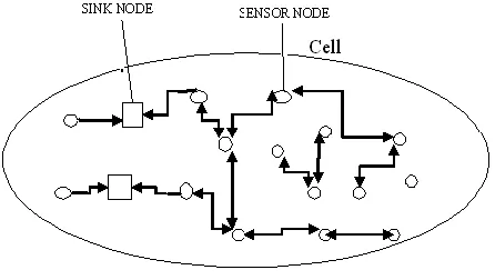
The general model for the network and traffic flowing through the network allowing for multicast of data generated at the sensor nodes to a set of sink nodes. This scenario can be useful in sensor networks. But, our problem can be considered as a generalization of multihop wireless networks where sleep and wake option may or may not be there and modes may not be harvesting energy. We define a mode of the network as a possible combination of active links along with their transmit powers such that any node is communicating with only one other node over a half duplex channel. The source of energy and the energy harvesting device may be such that the energy cannot be generated at all times (e.g., a solar cell). Thus, we need efficient energy management policies to modify the energy consumption profile of the sensor node so as to achieve the desired objectives with the given energy harvesting source. It should be done in such a way that the node can perform satisfactorily for a long time, i.e., energy starvation at least, should not be the reason for the node to die. In our study of energy harvesting sensor networks, the motivating application is the estimation of a random field which is one of the canonical applications of sensor networks. In this application, the sensor nodes sense the random field periodically. After sensing, a node generates a packet (possibly after efficient compression). This packet needs to be transmitted to a central node, possibly via other sensor nodes.

In addition to the control of data transmission that is to be done on a typical wireless network, energy management at each of the nodes presents some new challenges. For instance, if the rate of energy harvesting of some nodes is less, then they will have to switch to power saving modes. Thus, in a network of energy harvesting sensor nodes, in addition to the scheduling of data transmission, scheduling of the power saving modes at the nodes also has to be done carefully. Routing, in a more narrow sense of the term, is often contrasted with bridging in its assumption that network addresses are structured and that similar addresses imply proximity within the network. Because structured addresses allow a single routing table entry to represent the route to a group of devices, structured addressing (routing, in the narrow sense) outperforms unstructured addressing (bridging) in large networks, and has become the dominant form of addressing on the Internet, though bridging is still widely used within localized environments.

We will then evaluate the performance of the two approaches using certain examples. The approaches discussed here also become computationally intractable for large networks. We will also present the results obtained using a suboptimal approach and algorithms. Link Price updating will be done using the following algorithm for all the proposed algorithms for solving the dual problem. This update algorithm follows from a sub-gradient algorithm used for non-differentiable functions. A distributed sub-gradient algorithm for joint congestion control, routing and scheduling is obtain to approach arbitrarily close to the optimum of the system problem. In this algorithm, optimal routing for a flow depending on the link prices is obtained using a distributed routing algorithm.

II. MODEL

(2)

International Journal of Emerging Technology and Advanced Engineering

67 The system is slotted. During slot

k

_{(defined as time}

interval



k k, 1



,i.e; a slot is unit of time) ,

x

k bits are generated by the sensor node. Although the sensor node may generate data as packets, arbitrary fragmentation of packets during transmission is allowed (Zigbee allows byte level fragmentation; arbitrary fragmentation provides a reasonable approximation). Thus, packet boundaries are not important and bit strings are considered. The bits x_k are eligible for transmission in



k1



st slot. We assume that

each node transmits with a constant power P.

[image:2.612.62.285.323.449.2]

Adaptive transmit power, modulation (and/or coding) available in some commercially available transceivers will be consider.

Fig 1: Multicast wireless sensor network

Let the set of nodes in the network be denoted by

N

and indexed by

n

= 1,..., N. All nodes within transmission range of a node are connected to it via a unidirectional edge, called link. The set of links is denoted by

L

and indexed by

l

= 1,…, L. The communication between a source and destination pair is known as a flow. The set of flows is denoted by

F

and indexed by

f

= 1,..., F.

Source and destination of flow,

f

are denoted by

s f

( )

and

d f

( )

respectively. Due to interference, links in a neighborhood may not transmit successfully at the same time. A set of links which can be activated simultaneously (with L dimensional power vector, PL), is called a mode.

The set of modes is denoted by

M

and indexed by

m

= 1,..., M. We assume that the channel fading is constant during the time interval under consideration. We also assume that the rate of the links in a mode will be a function of SINR. A mode gives an L dimensional rate

vector,

R

 

m

which defines the capacity of all the links when mode m is selected.

In our model, the rate of link

l

is

R m

_l

( )

if the link

l

is active in mode

m

; else

R m

_l

( )

= 0. The modes so obtained are also called independent sets. For a given transmit power vector and time invariant channel gains, these modes are constant. There are distributed algorithms available for

computing independent sets ([13], [14]). Let

a

_m



 

0,1

be thefraction of time mode

m

is active.

We initially consider a simplified model where the sensor nodes are always awake and perform sensing in all the slots. The data generated at each sensor node has to be sent to the fusion node through the network. But, the network may not be able to carry all the data originating at each sensor node. In such a case, we require a flow control mechanism at the sensor nodes so that each sensor node gets a fair share of the network resources. In order to ensure fairness, we maximize the minimum of the satisfied fractions of demand of the sensor nodes in the network. The ratio of net flow from a node to the fusion node to the node’s demanded rate is the satisfied fraction (λ) of demand for that node.

Data carried on link

l

of flow

f

is denoted by

x

_lf .

A

is an (N X L) Node-Link incidence matrix for the wireless

network, where

a

_nl



1

if node

n

transmits on link

l

;

1

nl

a

 

if node

n

receives on link

l

;

a

_nl



0

otherwise.

A X



f



Y

f (1)

Where A is node-link matrix,

X

f is an L dimensional vector which gives the data on various links for flow

f

,

and

Y

f is an N dimensional vector which gives the data generated/consumed by the nodes for the flow

f

_.The equality indicates that total flow into a node equals the total flow out of the node except when the node is a source node or a sink node. This has to be satisfied for all

f



F

at every node.

Note that

X

f



0

and

a



0.

(3)

International Journal of Emerging Technology and Advanced Engineering

68

Y

f for node

s f

( )

is

r

_f, for node

d f

( )

it is



r

_f

and is 0 for the remaining nodes, if the data rate allocated for flow

f

is defined as

r

_f. The largest possible fraction



of all demands should be satisfied.

( )

min

f

,

f s f

s f f

r

f

F

d

r





 



(2)

From the flow constraints we can solve the problem by using following assumptions

(a)Optimization Problem

Our objective function is

max

U



 λ

( )

(3)

Where

U

( )



is the sum of utilities of all the users, if



fraction of their flow is transmits.

As in and we consider the dual of this problem to facilitate distributed implementation.

(b)Lagrange-Dual of the Problem

Let

p

be the Lagrange Multiplier or the Price Vector for the links, of dimension L.

T

0

D

U

f

,

f F

max



  _

 









































X λ

( )

p

( )

p

X

M

a

(4)

Subject to: ( )

1,

.

f f

m m M

s f f

f

F

a

d

r

f

F









 





  



A X

Y

This problem can be further split into two sub-problems:

 

1 2

D

p

and D

p

.

(c)Link Price Update Algorithm

Link Price updating will be done using the following algorithm for all the proposed algorithms for solving the dual problem.

This update algorithm follows from a sub-gradient algorithm used for non-differentiable functions. Since the

dual function

D

 

p

is not differentiable, we can not use the usual gradient methods and hence the dual problem is

solved using sub-gradient

f fF





 

g(

p

)

M

a

X

of the dual

function,

D

 

p

at

p

.

Thus by sub gradient method we obtain the following algorithm for the link price adjustment



1 

 

_j f

 

f F

j



j









 



_











_









X

M



p

a

(5)

Where



_j is a +ve scalar step size in

j

th iteration. We take



_j





,



j

,i.e., constant step size.

Hence, the price for link

l

from

j

to

j



1

will be updated as follows:



1 



 



 



l l l l

p j

 

p j





x j



R j

 (6)

Where

p

_l

 

j

is the price of link

l

in

j

th iteration,

 

l

x j

is the aggregate flow on link

l

in

j

th iteration,

 

l

R j

is the capacity of the link

l

during

j

th iteration, and



is the link price step.

In this chapter we don’t consider power control and channel gains are constant. Thus

R j

_l

 

= C b/s if link

l

is active during

j

th iteration, else it is zero.

(4)

International Journal of Emerging Technology and Advanced Engineering

69 III. ALGORITHMS

Algorithm 1: Concave Utility Algorithm

Step 1: Every node has the knowledge of the links

attached to it. From

j

to

j



1

iteration, it updates the price of link

l

using the price update algorithm given as equation (3.10for routing, the optimal route or the minimum priced path is chosen for each of the flows. i.e.

* f

X

for unit source flow

f

,

 

f

F

. Thus the nodes are aware of the data on various links along with the link prices for flows passing through it.

Step 3: Total path cost (at given link prices) and the demand for each flow gives the total cost for supporting the demanded flow. Aggregate for all the flows is

_{s f}_{( )} _Rf* f F

d







p

.

This can be passed on to a root node for finding the optimal



by organizing the network in a spanning tree with a root node, which controls this parameter, and the remaining nodes attached to it. Every node has the knowledge of the price and the flows on the links attached to it. Leaf nodes sum the cost and pass it to the parent node. Every node up the chain adds the cost received from its child nodes with cost computed by itself and passes this to

its parent node. Source node for flow

f

,

s f

 

also forward its demand

d

_{s f}_{ }.

Step 4:

U

( )



is the sum of utilities of all the users if



fraction of their flow is transmitted. We take

U( )=



is a concave function. Now,

U ( )

1

2 





' .

Unique maximiser of

D

₁

 

p

is at

U ( )

_{s f}_{( )} _Rf*

f F

d











'

p

.

Hence, root node can obtain the network parameter

2 * ( )

1

2

f

s f R

f F

d













 

_











p



.

Root node is aware of the function

U

and it requires the total cost for supporting the demanded flow for computing



. Thus root node gets the required information and computes



. This can be disseminated to all source nodes.

Note:





d

_{s f}_{( )}



X

f* is the optimal routing vector of flow

f

.

Step 5: Depending on the link price vector

p

, a mode (independent set of links) is chosen. i.e. scheduling is done. Over the iterations, average is taken to get the vector

a

. For scheduling, we solve the second optimization sub problem.

Algorithm 2: Binary Lambda Algorithm

Steps 1 to 3 are same as Algorithm 1.

Step 4:

U( ) =



is a linear function which can be

taken as concave function. Now

U ( ) 1

'





. Hence, the first sub-problem can be written as

T

1 ( )

0

D

f f* s f f F

max

 

d

  _  







_





_







X λ

( )

p

X

( ) R 0

1

f f* s f f F

max



d

  _  







_





_







X λ

p

Subject to the constraints.

Hence, the aggregate price for all the flows

i.e. _{s f}_{( )} _Rf* f F

d







p

is greater than 1, then

1

D

( )

p

is maximized for





0

.

Thus the root node raises a flag and stops all source nodes from transmitting, else the entire demanded flow is

allowed. i.e.





1

maximizes

D

₁

( )

p

if

*

( )

1

f s f R f F

d









p

.

Average value of



is taken over the iterations.

(5)

International Journal of Emerging Technology and Advanced Engineering

70 The difference in the two algorithms is in step 4 which finds the optimal value of



which is the global parameter used for congestion control with proportional fairness. Concave Utility Algorithm finds the optimal value of



at every iteration which needs to be disseminated to all source nodes where as Binary Lambda Algorithm finds whether it is profitable for supporting the entire demand or not based on the current link prices and routing. It then either allows the complete flow demands or none.

This will require just one bit control information but will have burstyness in the flows. Thus there is a tradeoff between the two algorithms with respect to these two parameters.

IV. SIMULATION RESULTS

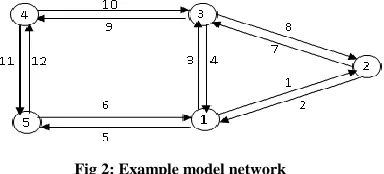
[image:5.612.368.503.184.442.2]

Take an example of a network having 5 nodes, 12 links and 6 flows and simulated both the proposed distributed algorithms

Fig 2: Example model network

Simulation Results for Concave Utility Algorithm

Here we are calculating the lambda which is nothing but fairness constraint. It is nothing but the ratio between the permissible data rate to the total transmission rate. The fairness of the sensor network will depends on the the value of lamda.As the value of lambda increases it indicates that permissible data rate of a flow is increased.

0 1000 2000 3000 4000 5000 6000 0.05

0.1 0.15 0.2 0.25 0.3 0.35 0.4

PLOT OF LAMBDA Vs NUMBER OF ITERATIONS

ITERATIONS

L

A

M

B

D

A

[image:5.612.78.270.366.453.2]

U(Lambda) = Fourth root of Lambda Link Price step = 0.001, Power Price step = 0.001 Harvested Power for all nodes = 0.5 units

Fig 3: Fairness graph

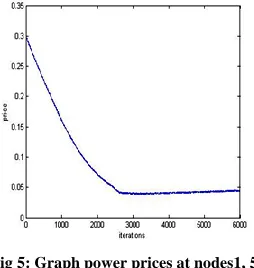
The following graphs will indicate the power prices that has been harvested at all the links which we have assumed, these graphs are plotted between the power price and the number of iterations.

Fig 4: Power prices graph for links1, 10

[image:5.612.72.258.555.694.2]

(6)

International Journal of Emerging Technology and Advanced Engineering

[image:6.612.106.233.144.278.2]

71

Fig 5: Graph power prices at nodes1, 5

Simulation Results for Binary Lambda algorithm:

Here also we are calculating the lambda which is nothing but fairness constraint.comparitively with the concave algorithm here link updation not perform upto some particular iteration. i.e. for more number of iteration only the link price reaches its maximum value that means fairness of the link increases.

Fig 6: Lambda graph (fairness graph)

Concave Utility Algorithm finds the optimal value of



at every iteration which needs to be disseminated to all source nodes where as Binary Lambda Algorithm finds whether it is profitable for supporting the entire demand or not based on the current link prices and routing. It then either allows the complete flow demands or none.

V. CONCLUSIONS AND FUTURE WORK

We optimized the power control, routing and scheduling for the network subject to the network constraints and proposed a distributed algorithm for solving the problem in an iterative manner. We compared the performance of the three approaches using examples. It solves the congestion problems in networks. So we may implement new congestion control methods to improve the fairness by using this method.

REFERENCES

[1] V. Joseph, V. Sharma and U. Mukherji, “Joint power control, scheduling and routing for multihop energy harvesting sensor networks,”2009, Submitted.

[2] V. Sharma, U. Mukherji, and V. Joseph, “Efficient energy management policies for networks with energy harvesting sensor nodes,” in Allerton Conference on Communication, Control, and Computing, 2008, Invited Paper.

[3] M. Kodialam, T. V. Lakshman, and S. Sengupta, Online multicast routing with bandwidth guarantees: a new approach using multicast network flow,” IEEE/ACM Trans. Netw., vol. 11, no. 4, pp. 676-686,2003.

[4] J. Yuan, Z. Li, W. Yu, and B. Li, “A cross-layer optimization framework for multihop multicast in wireless mesh networks,” IEEE Journal on Selected Areas in Communications, vol. 24, no. 11, pp. 2092-2103, Nov.2006

[5] Q. Cao, T. He, and T. Abdelzaher, “Ucast: Unified connectionless multicast for energy efficient content distribution in sensor networks,” IEEE Transactions on Parallel and Distributed Systems, vol. 18, no. 2, pp.240-250, Feb. 2007.

[6] Y. Wu, P. Chou, Q. Zhang, K. Jain, W. Zhu, and S.-Y. Kung, “Network planning in wireless ad hoc networks: a cross-layer approach,” IEEE Journal on Selected Areas in Communications, vol. 23, no. 1, pp. 136-150, Jan. 2005.

[7] M. Chiang, .To layer or not to layer: balancing transport and physical layers in wireless multihop networks, In Proc. of IEEE INFOCOM, 2004.

[8] L. Chen, S. H. Low, M. Chiang and J. C. Doyle, .Optimal cross-layer congestion control, routing and scheduling design in ad hoc wireless networks., In Proc. of IEEE INFOCOM, 2006.

[9] F. P. Kelly, A. K. Maulloo and D. K. H. Tan, .Rate control for communication networks: Shadow prices, proportional fairness and stability., Journal of Operations Research Society, 49(3):237-252, March 1998.

[10] S. H. Low, .A duality model of TCP and active queue management algorithms., IEEE/ACM Transactions on Networking, October 2003.

[11] X. Lin, N. Shroff, .Joint rate control and scheduling in multihop wireless networks., In Proc. of 43th IEEE CDC, 2004.

[image:6.612.50.292.378.564.2]