2016 International Conference on Mathematical, Computational and Statistical Sciences and Engineering (MCSSE 2016) ISBN: 978-1-60595-396-0
Improved I/O Data-Based Model-Free Adaptive Control
Technology in MIMO Discrete-Time Systems
Li-bo SONG
1,*, Yan-qiong FEI
2and Jin-song LI
11Engineering Training Center, Shanghai Jiao Tong University, 800 Dongchuan Rd., Shanghai, China
2School of Mechanical Engineering, Shanghai Jiao Tong University, 800 Dongchuan Rd., Shanghai,
China
*Corresponding author
Keywords: I/O data-based, Model-free adaptive control, MIMO, Discrete-time system.
Abstract. As one of I/O data-based model-free adaptive controllers, the conventional MFAC controllers only with zero-order output information of the system are widely used around the world. With the NARX model of the discrete-time system, the conventional MFAC controllers are reviewed based on some assumptions together with matrix-inversion-lemma and extreme value theory, parameter estimation method mathematically. On account of one-order output and a new weighted one-step-ahead control input cost function including one-order output, the new D-MFAC controller is obtained and its convergence is improved accordingly. Meanwhile, some simulations are made between the conventional MFAC controller and the D-MFAC controller with the same initial parameters in this paper. In result, the robust is proved and some conclusions are drawn.
Introduction
Comparing to model-based control methods based on the precise mathematical models, the new model-free adaptive control technique can stabilize the system without any model of the system. As a new control technology with self-learning capability, more and more studies focus on it to directly apply it to the complex processes whose dynamics with severe nonlinearities are poorly modeled.
There is a long developing process of MFAC control technique. Han and Wang started their primary research on the model-free control in the year 1994 and they proved the stability of this new method[1,2]. Since Hou expressed the fundamental frameworks of model-free adaptive control technology in his Ph.D thesis[3] and one of his books[4], and Cheng presented a kind of model-free adaptive control in his Ph.D thesis[4], there are some fruitful achievements in recent 10 years.
The MFAC theory is mature fundamentally and some MFAC controllers are implemented around the world, it has also been utilized successfully in engineering. Hou and his team used it successfully in traffic flow control and lithium-ion battery health management with artificial neural network and extended Kalman filter algorithm[6]. The Cybosoft Inc. has developed some practical MFAC controllers to replace PID control method and to eliminate manual tuning and nonlinearity etc[7]. Moreover, MFAC controllers have been applied in electromagnetic system[8], lithium-ion battery health management [9] and mismatch power converters[10] to propagate its successful applications. At the same time, some improved MFAC technologies have been put forwards to enhance its functionality. Xu [11] used neural network and equivalent proportion link to enhance the flexibility of adjustable parameters and speed, Dong [12] utilized a neural network as function approximator to improve the control performances and Zhao [13] present the improved MFAC with the modified control law and free of integral item, but these improved MFAC used the zero-order output data only. In order to use high-order output data like what in PID control, Liu [14] introduced a new MFAC with one-order output data, the convergence was proved.
of D-MFAC controller for controlling a differential-driven mobile robot are presented and conclusions are drawn in section 4.
The new D-MFAC controller
In view of convenience of description, the adaptive control of the following general discrete single-input and single-output (SISO) nonlinear system is considered first,
k
f
y
k y
k ny
u
k u
k un
y 1 ,, , ,, (1)
Where, y
k and u
k are the sets of outputs and control inputs of the discrete time k, f
is an unknown general nonlinear function, nyand nuare the orders of system output y
k and input u
krespectively. The Equation (1) can be called NARX model of the system generally. The following assumptions are considered about the nonlinear discrete time system: (A1)the partial derivative of f
with respect to control input u
k is continuous(A2)the system is generalized Lipschitz , that is to say, y
k1
bu
k for any k and
0u k with u
k1
u k1
u k , y
k1
y k1
y k and b is a positive constant and(A3)the system is controllable and observable and the control inputs and outputs are also bounded To get the input u
k , a weighted one-step-ahead control input cost function is given by
2
21
1
k u k u k
y k
y k u
J (2) Where, y
k1
is the expected system output and is a positive weighted constantMeanwhile, the cost function for parameter estimation proposed in many papers is used as
2
2 ˆ 11 k u k k k
k y k y k
J (3)
Where,
k and ˆ
k are the actual pseudo-partial derivative and the estimation value respectively. From three assumptions above, the system denoted by Equation (1) can be rewritten
k
y k k u ky 1 ˆ (4) Substituting Equation (4) into Equation (2) and Equation (3), and solving the equations
0J u k u k and J
k
k 0using the matrix-inversion-lemma and EVT, thus the control law u
k and the parameter estimation ˆ
k can be obtained respectively. Summarizing, the conventional MFAC controller in compact form can be given as follows:
k k
k
k y k
y k k
k k
u
k u k k y k
u k
u k u k
T T
u or ˆ
if
0 ˆ ˆ
1 ˆ
ˆ ˆ
1 1
ˆ 1
1 1 ˆ
(5)
Where, ,
0,2 are the step size, , are the weighted factors, is a small positive constant,
0ˆ
Motivation for the new MFAC controller is to use one-order term of output disappearing in the conventional MFAC equations. When the one-order output information y
k is replaced by the following equation
k dy
k dt
y
k
y k
dTy 1 (6) Where, dT is the sample time of the system. If the new weighted one-step-ahead control input cost function J
u
k
is rewritten as follows when y
k is incorporated
2
2
21 1
1
1 y k u k u k y k y k dT
k y k u
J (7) To incorporate the one-order term y
k into the cost function, the new weighted one-step-ahead control input cost function J
u
k
shown in Equation (7) can be rewritten as
2
21 1
1
k u k u k y k y k u J
21
1 u k k u k dT
k
(8) Using the extreme value theory and solving the equation J
u
k
u k 0 and we can get the new input u
k . With the same procedure and the same cost function for parameter estimation as Equation (3), then the improved MFAC controller can be written as following,
1
22 2 2 2 2 2 or ˆ if 0 ˆ ˆ 1 1 ˆ 1 1 ˆ ˆ 1 1 ˆ ˆ 1 1 ˆ k u k k k u k k y k u k u k k dT k u k k dT k y k y k k u (9)
Where, is a positive parameter used to adjust the function of one-order output y
k in the control approach. Hence, it can be called adjusting coefficient. If 0, the Equation (9) is the conventional MFAC technology, otherwise, it is the D-MFAC when 1 just because the one-order output is included like what in the PID control method. Normally, 1 2 .The error e
k1
between the actual output y
k1
and the desired output y
k1
can be defined as e
k1
y
k1
y k1
. In a SISO system, it can be known that the error
k1
y
k1
yk k
uk uk1
e
k e
k dT k k k e k dT k k k e T T 2 2 22 1 ˆ
ˆ 1 ˆ 1 ˆ
k e
kk k T 2 ˆ ˆ 1 (10)
The Equation (9) implies that the matrix
k ˆT k
1ˆ ˆ 1
0 2
k k
k T
(11)
by selecting the proper controller parameters and because
k and ˆ
k are bounded. Hence, the Eq.(10) can be deduced by taking norm of it,
0 ˆˆ 1
1 2 e k e k 1e
k k k k
e k
T
(12)
With the proper initial error e
0 and the positive constant and consequently the next equation can be obtained,
1
lim
0 0lim 1
e k e
k k
k (13)
It is so clear that the error e
k1
can be convergent to 0 when these proper control parameters areselected for the system, and the system can be stabilized to the desired output y
k1
driven by the new D-MFAC controller shown above as the Equation (9).Simulations
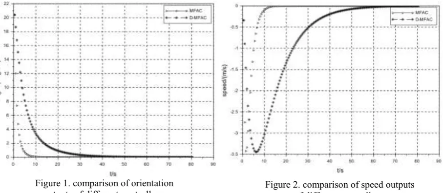
Some parameters are initialized as follows, 0.5, 0.8, 0.3,0.5 , y
0
0.2 1
T,
Ty1 1 0.2 , y
2
7.5 0.1
T , u
0
0 0.1
T , u
1
0.1 1
T , u
2
0.1 0.1
T ,
T10 75 . 0 ; 8 . 0 10 0
,
1
8 1;1 7
T ,
2
6 1;1 5
T and the desired output of the system is y
28 0.26
T. Where, the sign T means Matrix Transposition mathematically. And the sample time is set as dT0.5 to reduce computations and 0.00005 ordinarily. Using the free software SciLAB V5.5.1, some simulations are made to compare the D-MFAC controller with the conventional MFAC controller. Under circumstance of the same initial parameters, the comparison of orientation outputs and speed outputs are illustrated in Fig.1 and Fig.2 respectively.It is illustrated that 1) two outputs, the orientation output and the speed output, of the D-MFAC controller can be convergent to the desired outputs, 2) the D-MFAC controller stabilizes the system slower than the conventional MFAC controller due to smaller control inputs, and there is longer stabilizing time needed for the D-MFAC controller, 3) the amplitude of overshoot of speed in the
[image:4.595.80.534.510.708.2]Figure 2. comparison of speed outputs of different controllers. Figure 1. comparison of orientation
D-MFAC controller is similar to the conventional MFAC controller, and there is no significant reduction of overshoots in the D-MFAC controller.
Summary
On basis of linearization method, extreme value theory and parameter estimation method, the nonlinear discrete-time D-MFAC controller in the compact form is derived from the NARX model when a new weighted one-step-ahead control input cost function including one-order term of output is adopted in this paper. With some simulations it illustrated mainly with the same initial parameters that 1) the system can be stabilized with the new D-MFAC controller in slower speed and longer settling time with the D-MFAC controller than that of the conventional MFAC controller with the same initial parameters normally, 2) there are overshoots in the D-MFAC controller which can not be reduced significantly.
Next, we will focus on the method how to settle and stable the system faster with the D-MFAC controller, and realize it on some 8-bit MCU controllers to control the wheeled mobile robots.
Acknowledgement
This research was financially supported by the National Natural Science Foundation of China.
References
[1]Z.G. Han, D.J. Wang, Controller without model. Journal of Natural Science of Heilong-Jiang University.4(1994) 29-35.nes and Control.3(2006) 333-335.
[3]Z.S. Hou, The Parameter Identification, Adaptive Control and Model Free Learning Adaptive Control for Nonlinear Systems, Shenyang, 1994.
[4]Z.S. Hou, Non-parameteral model and its adaptive control theory, Beijing, 2000.
[5]S.X. Cheng, Model-free adaptive control theory and applications, Shanghai, 1996.
[6]R.H. Cai, Z.S. Hou, A model-free adaptive control approach for freeway traffic density via ramp metering, International Journal of Innovative Computing, Information and Control.11(2008) 2823-2832.
[7]Information on http://industrial.embedded-computing.com/pdfs/Cybosoft.Spr06.pdf
[8]A. Javadi, S. Pezeshki, A new model-free adaptive controller versus non-linear H controller for levitation of an electromagnetic system, Transactions of the Institute of Measurement and Control.3(2012)321-329.
[9]G.X. Bai, P.F. Wang, C. Hu et al. A generic model-free approach for lithium-ion battery health management. Applied Energy.135(2014)247-260.
[10]J.H. Wu, H.T. Yang and H.X. Zhang et al. Model-free Adaptive Control for Model Mismatch Power Converters, Chinese Control and Desicion Conference. 1(2011)1168-1171.
[11]A.D. Xu, Y.B. Zheng and Y.Song et al, An Improved Model Free Adaptive Control Algorithm, Fifth International Conference on Natural Computation.1(2009)70-74.
[12]N. Dong, A.G. Wu, Z.Q. Chen, Improved adaptive data-driven control for discrete nonlinear systems, Control Theory & Applications. 30(2013)1309-1314.
[13]Y. Zhao, C. Lu and Y.D. Han etal, Wide area power system stabilizer design based on improved model free adaptive control, Journal of Tsinghua University. 53(2013)1645-1652.