On the preconditioned GAOR method for a linear complementarity problem with an M matrix

R E S E A R C H

Open Access

On the preconditioned GAOR method for

a linear complementarity problem with an

M-matrix

Shu-Xin Miao

_{and Dan Zhang}

*_{Correspondence:}

[email protected]

1_{College of Mathematics and}

Statistics, Northwest Normal University, Lanzhou, People’s Republic of China

Abstract

Recently, based on the Hadjidimos preconditioner, a preconditioned GAOR method was proposed for solving the linear complementarity problem (Liu and Li in East Asian J. Appl. Math. 2:94–107,2012). In this paper, we propose a new preconditioned GAOR method for solving the linear complementarity problem with anM-matrix. The convergence of the proposed method is analyzed, and the comparison results are obtained to show it accelerates the convergence of the original GAOR method and the preconditioned GAOR method in (Liu and Li in East Asian J. Appl. Math. 2:94–107, 2012). Numerical examples verify the theoretical analysis.

MSC: 65F10; 65F15

Keywords: Linear complementarity problem; Preconditioner; Preconditioned GAOR method;M-matrix

1 Introduction

For a given matrixA∈Rn×n_{and a vectorf ∈R}n_{, the linear complementarity problem,} abbreviated as LCP, consists of finding a vectorx∈Rn_{such that}

x≥0, r:=Ax–f ≥0, and xTr= 0. (1) Here, the notation “≥” denotes the componentwise defined partial ordering between two vectors and the superscriptTdenotes the transpose of a vector.

The LCP of the form (1) arises in many scientific computing and engineering applica-tions, for example, the Nash equilibrium point of a bimatrix game, the contact problem, and the free boundary problem for journal bearings; see [5,16] and the references therein. As is known, LCP (1) possesses a unique solution if and only ifA∈Rn×n_{is aP-matrix,} namely a matrix whose all principal submatrices have positive determinants; see [4,5, 16]. A matrixAis called anM-matrix if its inverse is nonnegative and all its off-diagonal entries are nonpositive. A positive diagonalM-matrix is aP-matrix, and LCP (1) with an

M-matrix has the unique solution [3].

Because of the wide applications, the research on the numerical methods for solving (1) has attracted much attention. There are some iterative methods for obtaining the solution of the LCP, including the projected methods [8,9,12], the modulus algorithms [10], and

the modulus-based matrix splitting iterative methods [2,6,18,19], see [9] for a survey of the iterative method for LCP (1). We consider the generalized AOR (GAOR) method [8,12], which is a special case of the projected method, for solving LCP (1) with anM -matrix. For accelerating the convergence rate of the GAOR method, the preconditioned GAOR method is proposed in [13], based on the preconditioner in [7], for LCP (1) with an

M-matrix. In this paper, a new preconditioner is proposed to accelerate the convergence rate of the GAOR method for solving LCP (1).

The outline of the rest of the paper is as follows. In Sect.2, some preliminaries about the projected method are reviewed, and the new preconditioner for preconditioned GAOR method is introduced. Convergence analysis is given in Sect.3. The convergence rates of the proposed preconditioned GAOR method are compared with the convergence rates of the preconditioned GAOR method in [13] and the convergence rates of the original GAOR method for LCP with anM-matrix in Sect.4, which shows that the proposed precondi-tioned GAOR converges faster than the precondiprecondi-tioned GAOR method in [13] and the original GAOR method. Numerical examples are given to verify the theoretical results in Sect.5. Finally, conclusions are drawn in Sect.6.

2 Preliminaries

We give some of the notations, definitions, and lemmas which will be used in the sequel. ForA= (ai,j),B= (bi,j)∈Rn×n, we writeA≥Bifai,j≥bi,jholds for alli,j= 1, 2, . . . ,n.A≥O is called nonnegative ifai,j≥0 for alli,j= 1, 2, . . . ,n, whereOis ann×nzero matrix. For the vectorsa,b∈Rn×1_{,a≥banda≥0 can be defined in a similar manner. By|A|= (|a}

ij|) we define the absolute value of a given matrixA∈Rn×n_{. We denote then×ndiagonal} matrix coinciding in its diagonal with matrixC∈Rn×n_{bydiag(C). For simplicity, we may} assume thataii= 1 (i= 1, 2 . . .n).

Lemma 1([17]) Let A= [aij]∈Rn×nand aij≤0for i=j.A is an M-matrix if and only if

there exists a positive vector y such that Ay> 0.

There are equivalent conditions of anM-matrix, a nonsingularM-matrix is a monotone matrix, see [4].

Definition 1([4]) For a matrixA∈Rn×n, the representationA=M–Nis called a splitting

ofAifMis nonsingular. ThenA=M–Nis called weak regular ifM–1≥0 andM–1N≥0. For the weak regular splittings of different monotone matrices, there is a comparison result as follows.

Lemma 2([4]) Suppose that A1=M1–N1and A2=M2–N2are weak regular splittings

of the monotone matrices A1 and A2,respectively,such that M–11 ≤M2–1.If M1–1N1 has a

positive Perron vector,then

ρM–1₂ N2

≤ρM–1₁ N1

.

The following lemma is taken from [11].

Lemma 3([11]) Let A be an M-matrix and x be a solution of LCP(1).If fi> 0,then xi> 0

For the study of the projected methods, the following definition is needed.

Definition 2([15]) Given any vectorx∈Rn_,x

+denotes the vector with components

(x+)i=max{xi, 0} ∀i∈N:={1, 2, . . . ,n}.

From Definition2, the following properties hold for anyx,y∈Rn_: (i) (x+y)+≤x++y+;

(ii) x+–y+≤(x–y)+;

(iii) |x|=x++ (–x)+;

(iv) x≤y⇒x+≤y+.

Using Definition2, LCP (1) is analogous to [1]

x=x–D–1(Ax–f)₊, (2)

whereD=diag(A) is a nonsingular matrix. From (2) and the splitting ofAasA=D–L–U, hereD, –L, –Uare the diagonal, the strictly lower, and the strictly upper triangular parts of A, respectively. The GAOR method for solving (1) can be defined as (see [8,12])

xk+1=xk–D–1αLxk+1+ (A–αL)xk–f₊, k= 0, 1, . . . , (3)

where=diag(ω1,ω2, . . . ,ωn) is a positive diagonal matrix andαis a positive real number. LetJ=D–1_{(L+U),G=I–αD}–1_{|L|, andF=|I–D}–1_{(A–αL)|, the following result} concerns the convergence of the GAOR method for solving LCP (1).

Lemma 4([12]) Suppose that A is a positive diagonal H-matrix.Then,for any initial

vec-tor x0∈Rn,the iterative sequence{xk}generated by the GAOR method(3)converges to the unique solution x∗of LCP(1),and

ρG–1F≤max

1≤i≤n

|1 –ωi|+ωiρ

|J|< 1,

where0 <ωi< 2/[1 +ρ(|J|)]and0≤α≤1.

For accelerating the convergence rate of the GAOR method, a preconditioner, based on the Hadjidimos preconditioner [7], is proposed in [13]

P=

⎡ ⎢ ⎢ ⎢ ⎢ ⎢ ⎢ ⎢ ⎢ ⎢ ⎢ ⎣

1

–γ2a21–β2 1 ..

. . ..

–γiai1–βi 1 ..

. . ..

–γnan1–βn 1

⎤ ⎥ ⎥ ⎥ ⎥ ⎥ ⎥ ⎥ ⎥ ⎥ ⎥ ⎦

,

equivalent linear complementarity problem of LCP (1)

x≥0, ˜r=Ax˜ –Pf˜ ≥0, xT˜r= 0

has the unique solution [3]. The preconditioned GAOR method for solving LCP (1) is defined [13] as

xk+1=xk–D–1αLxk+1+ (A–αL)xk–Pf₊, k= 0, 1, . . . , (4) based on the splittingA=D–L–U, please refer to [13] for more details.

Note that the preconditioning effect ofPis not observed on the first row of matrixA. In order to provide the preconditioning effect on all the rows ofA, in this paper, we propose the following preconditioner:

P=

⎡ ⎢ ⎢ ⎢ ⎢ ⎢ ⎢ ⎢ ⎢ ⎢ ⎢ ⎣

1 –γ1a1n–β1

–γ2a21–β2 1 ..

. . ..

–γiai1–βi 1 ..

. . ..

–γnan1–βn 1

⎤ ⎥ ⎥ ⎥ ⎥ ⎥ ⎥ ⎥ ⎥ ⎥ ⎥ ⎦

, (5)

whereγi≥0 (i= 1, . . . ,n) andβi(i= 1, . . . ,n) are constants.

Let the preconditioned matrixA=PAbe split asA=D–L–U, whereD,L, andUare the diagonal, lower triangular, and upper triangular matrices, then the preconditioner GAOR method for solving LCP (1) is defined as

xk+1=xk–D–1αLxk+1+ (A–αL)xk–Pf₊, k= 0, 1, . . . . (6) 3 Convergence analysis

In this section, we will consider the convergence of the preconditioned GAOR method (6) for solving LCP (1). In what follows, we make the assumptions:

(H0) f1> 0andfn> 0;

(H1) 0≤γi≤1fori= 1, 2, . . . ,n; (H2) –γ1a1n+a1n≤β1≤–γ1a1n;

(H3) –γiai1+ai1≤βi≤–γiai1fori= 2, 3, . . . ,n.

Theorem 1 LetA=PA= [aˆij]andfˆ=Pf = [fˆi].If (H0)–(H3)are satisfied,then LCP(1)is

equivalent to the linear complementarity problem

x≥0, ˆr=Axˆ –fˆ≥0, xTrˆ= 0. (7)

Proof After some calculations, the elements ofAandf can be expressed, respectively, as follows:

ˆ

aij=

⎧ ⎨ ⎩

a1j– (γ1a1n+β1)anj, i= 1,j= 1, 2, . . . ,n,

aij– (γiai1+βi)a1j, i= 1,j= 1, 2, . . . ,n,

and

ˆ

fi=

⎧ ⎨ ⎩

f1– (γ1a1n+β1)fn, i= 1,

fi– (γiai1+βi)f1, i= 1.

(9)

Letxbe a solution of LCP (1). Sincef1> 0 andfn> 0, from Lemma3we havex1> 0,

n

j=1a1jxj–f1= 0, andxn> 0,

n

j=1anjxj–fn= 0. Therefore, on the one hand, ifi= 1, then

n

j=1 ˆ

aijxj–fˆi= n

j=1

a1j– (γ1a1n+β1)anj

xj–

f1– (γ1a1n+β1)fn

= n

j=1

a1jxj–f1– (γ1a1n+β1)

_n

j=1

anjxj–fn

= n

j=1

a1jxj–f1. (10)

On the other hand, ifi= 1, then

n

j=1 ˆ

aijxj–fˆi= n

j=1

aij– (γiai1+βi)a1j

xj–

fi– (γiai1+βi)f1

= n

j=1

aijxj–fi– (γiai1+βi)

_n

j=1

a1jxj–f1

= n

j=1

aijxj–fi. (11)

Thus,xis a solution of LCP (7).

Conversely, suppose thatxis the solution to LCP (7), assumptions (H0), (H3) and (9) imply thatβn+γnan1≤0, so –(βn+γnan1)f1≥0, thenfn– (βn+γnan1)f1≥0, we get that ˆ

fn> 0. Similarly, from assumptions (H0), (H2) and (9), we can obtainfˆ1> 0. It follows from Lemma3thatx1> 0,

n

j=1aˆ1jxj–fˆ1= 0, andxn> 0,

n

j=1aˆnjxj–fˆn= 0. This together with (10) and (11) givesn_j=1aijxj–fi= 0. Thus, fori= 1, we have

n

j=1

(aijxj–fi) = n

j=1

(aijxj–fi) – (γ1a1n+β1)

_n

j=1

anjxj–fn

= n j=1

a1j– (γ1a1n+β1)anj

xj–

f1– (γ1a1n+β1)fn

= n j=1 ˆ

While fori= 1, we can deduce that

n

j=1

(aijxj–fi) = n

j=1

(aijxj–fi) – (γiain+βi)

_n

j=1

a1jxj–f1

= n

j=1

aij– (γiai1+βi)a1j

xj–

fi– (γiai1+βi)f1

= n

j=1 ˆ

aijxj–fˆi.

Hence,xis the solution of LCP (1).

Lemma 5 If A is an M-matrix, (H1)–(H3)hold,thenA=PA is an M-matrix.

Proof IfAis anM-matrix, thenaij< 0 fori=janda1iai1< 1, which leads toa1i> 1/ai1. Otherwise, from (8) and assumption (H2), –γ1a1n+a1n≤β1≤–γ1a1n, we have thatβ1+

γ1a1n≤0 andβ1+γ1a1n≥a1n> 1/an1. Thenaˆ11=a11– (β1+γ1a1n)an1> 1 – 1/an1∗an1= 0. Similarly, we can obtain

ˆ

a11=a11– (γ1a1n+β1)an1> 0, ˆ

aii=aii– (γiai1+βi)a1i> 0, i= 1, ˆ

a1j=a1j– (γ1a1n+β1)anj< 0, ˆ

aij=aij– (γiai1+βi)a1j< 0, i= 1,j.

From Lemma1there exists a positive vectory> 0 such thatAy> 0. Note thatP> 0, thus

Ay=PAy> 0, and from Lemma1,Ais anM-matrix.

Theorem 2 Let A be a diagonally dominant M-matrix.If (H0)–(H3)hold,then for0≤

ωi≤2/[1 +ρ(|ˆJ|)] (i= 1, . . . ,n)and0≤α≤1,the iterative sequence of the preconditioned

GAOR method(6)converges to the unique solution x∗of LCP(1),hereJˆ=D–1_(L+U).

Proof From Lemma5, we know thatAis a diagonally dominantH-matrix. Thus from Theorem1and Lemma4, the preconditioned GAOR method (6) converges to the unique

solution of LCP (1).

4 Comparison results

In this section, we will compare the convergence rate of the preconditioned GAOR method (6) with that of the GAOR method (3) and that of the preconditioned GAOR method (4) [13]. For simplicity, we may assume thataii= 1,i= 1, . . . ,n. For this case,G=I–α|L|,

U=U+SUwith S= ⎡ ⎢ ⎢ ⎢ ⎢ ⎢ ⎢ ⎢ ⎢ ⎢ ⎢ ⎣ 0

–γ2a21–β2 0 ..

. . ..

–γiai1–βi 0 ..

. . ..

–γnan1–βn 0

⎤ ⎥ ⎥ ⎥ ⎥ ⎥ ⎥ ⎥ ⎥ ⎥ ⎥ ⎦ ,

SD=

⎡ ⎢ ⎢ ⎢ ⎢ ⎢ ⎢ ⎢ ⎣ 0

(γ2a21+β2)a12

(γ3a31+β3)a13 . ..

(γnan1+βn)a1n

⎤ ⎥ ⎥ ⎥ ⎥ ⎥ ⎥ ⎥ ⎦ ,

SL=

⎡ ⎢ ⎢ ⎢ ⎢ ⎢ ⎢ ⎢ ⎣

0 0 · · · 0 0

0 0 · · · 0 0

0 (γ3a31+β3)a12 · · · 0 0

..

. ... . .. ... ...

0 (γnan1+βn)a12 · · · (γnan1+βn)a1,n–1 0

⎤ ⎥ ⎥ ⎥ ⎥ ⎥ ⎥ ⎥ ⎦ ,

SU=

⎡ ⎢ ⎢ ⎢ ⎢ ⎢ ⎢ ⎢ ⎣

0 0 · · · 0 0

0 0 (γ2a21+β2)a13 · · · (γ2a21+β2)a1n ..

. ... . .. ... ...

0 0 0 · · · (γn–1an–1,1+βn–1)a1n

0 0 0 · · · 0

⎤ ⎥ ⎥ ⎥ ⎥ ⎥ ⎥ ⎥ ⎦ .

Moreover, theD,L, andUcan be expressed asD=I–SD–RD,L=L–S+SL,U=U+

SU–R+RUwith

R= ⎡ ⎢ ⎢ ⎢ ⎢ ⎣

0 · · · 0 –γ1a1n–β1

0 · · · 0 0

..

. . .. ... ...

0 · · · 0 0

⎤ ⎥ ⎥ ⎥ ⎥ ⎦,

RD=

⎡ ⎢ ⎢ ⎢ ⎢ ⎣

(γ1a1n+β1)an1 0 . .. 0 ⎤ ⎥ ⎥ ⎥ ⎥ ⎦,

RU=

⎡ ⎢ ⎢ ⎢ ⎢ ⎣

0 (γ1a1n+β1)an2 · · · (γ1a1n+β1)ann

0 0 · · · 0

..

. ... . .. ...

0 0 · · · 0

⎤ ⎥ ⎥ ⎥ ⎥ ⎦.

Proof Note that

D=diag1, 1 – (γ2a21+β2)a12, . . . , 1 – (γnan1+βn)a1n

and

D=diag1 – (γ1a1n+β1)an1, 1 – (γ2a21+β2)a12, . . . , 1 – (γnan1+βn)a1n

.

SinceAis anM-matrix with diagonal elements 1, we have 0 <aijaji< 1 (i=j) [7]. Then assumptions (H1)–(H3) imply that

0 < 1 – (γ1a1n+β1)an1< 1

and

0 < 1 – (γiai1+βi)a1i< 1, i= 2, . . . ,n.

Hence, 0≤D≤D.

From Lemma6and the fact thatL=L, we have

D–1|L| ≤D–1|L|. (12)

Moreover, it is easy to check that the inequality

|L| ≤D–1|L| (13)

holds [14]. LetG=I–αD–1|L|,F=|I–D–1(A–αL)|,G=I–αD–1|L|, andF= |I–D–1_{(A–αL)|. If (H1) and (H3) hold, then [14]}

ρ G–1F≤ρG–1F< 1. (14)

The following theorem gives a comparison result betweenρ(G–1_{F) withρ(G}–1_F).

Theorem 3 If A is an irreducible nonsingular M-matrix,and(H0)–(H3)hold,then

ρG–1F≤ρ G–1F< 1.

Proof It follows from Theorem2and (14) thatρ(G–1_{F) < 1 andρ(G}–1_{F) < 1, so we only} need to show

ρG–1F≤ρ G–1F. In terms of (12), we have

that is,G≤G. Note thatGandGareM-matrices, hence

0≤G–1≤G–1. (15)

AsF=|I–D–1_{(A–αL)|andF=|I–D}–1_{(A–αL)|are nonnegative matrices, thus,} this together with (15) yieldsG–FandG–Fare the regular splitting of different monotone matricesG–FandG–F, respectively. Moreover, for a nonnegative matrixG–1_{F, according} to Perron–Frobenius theorem (see [4]), there is a positive Perron vectorzsuch that

G–1Fz=ρ G–1Fz.

Hence, it follows from Lemma2that

ρG–1F≤ρ G–1F.

The proof is completed.

Remark1 From Theorem3and (14), we can see that under assumptions (H0)–(H3), the inequalities

ρG–1F≤ρ G–1F≤ρG–1F< 1

hold. This confirms that the proposed preconditionerPin (5) is more efficient than the preconditionerP[13] for accelerating the convergence rate of GAOR method for solving LCP (1) with anM-matrix.

5 Numerical example

In this section, two examples are given for verifying the theoretical result.

Example1 Linear complementarity problem with coefficient matrix

A1=

⎡ ⎢ ⎢ ⎢ ⎢ ⎢ ⎢ ⎣

1.00000 –0.00580 –0.19350 –0.25471 –0.03885 –0.28424 1.00000 –0.16748 –0.21780 –0.21577 –0.24764 –0.26973 1.00000 –0.18723 –0.08949 –0.13880 –0.01165 –0.25120 1.00000 –0.13236 –0.25809 –0.08162 –0.13940 –0.04890 1.00000

⎤ ⎥ ⎥ ⎥ ⎥ ⎥ ⎥ ⎦

.

Tables1and2listρ(G–1F),ρ(G–1F), andρ(G–1F) for differentαand.

Table 1 ρ(G–1_F),ρ(G–1_{F), andρ(G}–1_{F) withα= 0.1 andω} i= 0.1

Preconditioner (γ1,. . .,γ5)T (β1,. . .,β5)T ρ(·)

I – – 0.96934

P (0, 1, 1, 1, 0.1)T _{(0, 0.1, 0, 0.01, 0.05)}T _0.96311

(0, 1, 0, 1, 0)T _{(0, 0, 0.04, 0.04, 0.05)}T _0.96750

P (1, 1, 1, 1, 0.1)T _{(0.03, 0.1, 0, 0.01, 0.05)}T _0.96292

Table 2 ρ(G–1F),ρ(G–1F), andρ(G–1F) withα= 0.1 andωi= 0.9

Preconditioner (γ1,. . .,γ5)T (β1,. . .,β5)T ρ(·)

I – – 0.71690

P (0, 1, 1, 1, 0.1)T _{(0, 0.1, 0, 0.01, 0.05)}T _0.67388

(0, 1, 0, 1, 0)T _{(0, 0, 0.04, 0.04, 0.05)}T _0.70036

P (1, 1, 1, 1, 0.1)T _{(0.03, 0.1, 0, 0.01, 0.05)}T _0.67153

(1, 1, 0, 1, 0)T _{(0, 0, 0.04, 0.04, 0.05)}T _0.69654

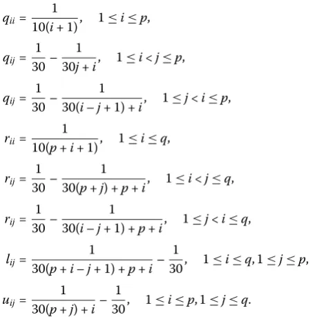
Example2 Let the coefficient matrixAof LCP (1) be given by

A=

I–Q U L I–R

,

whereQ= (qij)∈Rp×p,R= (rij)∈Rq×q,L= (lij)∈Rq×p, andU= (uij)∈Rp×qwith

qii= 1

10(i+ 1), 1≤i≤p,

qij= 1 30–

1

30j+i, 1≤i<j≤p, qij=

1 30–

1

30(i–j+ 1) +i, 1≤j<i≤p, rii=

1

10(p+i+ 1), 1≤i≤q,

rij= 1 30–

1

30(p+j) +p+i, 1≤i<j≤q, rij=

1 30–

1

30(i–j+ 1) +p+i, 1≤j<i≤q, lij=

1

30(p+i–j+ 1) +p+i–

1

30, 1≤i≤q, 1≤j≤p,

uij= 1 30(p+j) +i–

1

30, 1≤i≤p, 1≤j≤q. It is obvious thatAis an irreducibleM-matrix.

Table3and Table4listρ(G–1_F),ρ(G–1_{F), andρ(G}ˆ–1_Fˆ_{) with differentαandfor} Exam-ple2, where inP˜, let (γ1,γ2, . . . ,γn)T= (0,1₃, . . . ,1₃)T, (β1,β1, . . . ,βn)T= (0, 0.003, . . . , 0.003)T and in Pˆ, let (γ1,γ2, . . . ,γn)T = (1₃,1₃, . . . ,1₃)T, (β1,β1, . . . ,βn)T = (0.003, 0.003, . . . , 0.003)T.

Table 3 ρ(G–1F),ρ(G–1F), andρ(Gˆ–1Fˆ) withα= 0.1 andωi= 0.6 for Example2

n I P˜ Pˆ

5 0.46078 0.46040 0.46038

10 0.55689 0.55636 0.55635

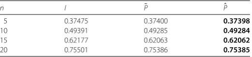
15 0.65889 0.65833 0.65832

Table 4 ρ(G–1F),ρ(G–1F), andρ(Gˆ–1Fˆ) withα= 0.2 andωi= 0.7 for Example2

n I ˜P Pˆ

5 0.37475 0.37400 0.37398

10 0.49391 0.49285 0.49284

15 0.62177 0.62063 0.62062

20 0.75501 0.75386 0.75385

From Tables1,2,3, and4we can see that, for different choices ofαand, the inequalities

ρG–1F≤ρ G–1F< 1

hold, which verifies the theoretical result in Theorem3.

6 Conclusions

In this paper, we present a new preconditionerP, which provides the preconditioning effect on all the rows of A, to accelerate the convergence rate of the GAOR method to solve LCP (1) with anM-matrixA, and consider the preconditioned GAOR method (6). We prove that the original LCP (1) is equivalent to LCP (7), and show that the precondi-tioned GAOR method (6) is convergent for solving LCP (1). Then a comparison theorem on the preconditioned GAOR method (6) is obtained, which shows that the precondi-tioned GAOR method (6) improves the convergence rate of the precondiprecondi-tioned GAOR method in [13] for solving LCP (1). Together with the comparison result in [12], we know that the preconditioned GAOR method (6) improves considerably the convergence rate of the original GAOR method for solving LCP (1).

Acknowledgements

The authors would like to thank the editors and reviewers for their valuable comments, which greatly improved the readability of this paper.

Funding

This paper is supported by the China Postdoctoral Science Foundation (No.2017M613244).

Competing interests

The authors declare that they have no competing interests.

Authors’ contributions

All authors contributed equally to the writing of this paper. All authors read and approved the final manuscript.

Publisher’s Note

Springer Nature remains neutral with regard to jurisdictional claims in published maps and institutional affiliations.

Received: 18 March 2018 Accepted: 20 July 2018

References

1. Ahn, B.H.: Solution of nonsymmetric linear complementarity problems by iterative methods. J. Optim. Theory Appl. 33, 185–197 (1981)

2. Bai, Z.-Z.: Modulus-based matrix splitting iteration methods for linear complementarity problems. Numer. Linear Algebra Appl.17, 917–933 (2010)

3. Bai, Z.-Z., Evans, D.-J.: Matrix multisplitting relaxation methods for linear complementarity problems. Int. J. Comput. Math.63, 309–326 (1997)

4. Berman, A., Plemmons, R.J.: Nonnegative Matrices in the Mathematical Sciences. SIAM, Philadelphia (1994) 5. Cottle, R., Pang, J.-S., Stone, R.M.: The Linear Complementarity Problem. Academic Press, San Diego (1992) 6. Dong, J.-L., Jiang, M.-Q.: A modified modulus method for symmetric positive-definite linear complementarity

problems. Numer. Linear Algebra Appl.16, 129–143 (2009)

7. Hadjidimos, A., Noutsos, D., Tzoumas, M.: More on modifications and improvements of classical iterative schemes for

8. Hadjidimos, A., Tzoumas, M.: On the solution of the linear complementarity problem by the generalized accelerated overrelaxation iterative method. J. Optim. Theory Appl.165, 545–562 (2015)

9. Hadjidimos, A., Tzoumas, M.: The solution of the linear complementarity problem by the matrix analogue of the accelerated overrelaxation iterative method. Numer. Algorithms73, 665–684 (2016)

10. Kappel, N.W., Watson, L.T.: Iterative algorithms for the linear complementarity problems. Int. J. Comput. Math.19, 273–297 (1986)

11. Li, D.H., Zeng, J.P., Zhang, Z.: Gaussian pivoting method for solving linear complementarity problem. Appl. Math. J. Chin. Univ. Ser. B12, 419–426 (1997)

12. Li, Y., Dai, P.: Generalized AOR for linear complementarity problem. Appl. Math. Comput.188, 7–18 (2007) 13. Liu, C., Li, C.: A new preconditioned generalised AOR method for the linear complementarity problem based on a

generalised Hadjidimos preconditioner. East Asian J. Appl. Math.2, 94–107 (2012)

14. Liu, Y., Zhang, R., Wang, Y., Huang, X.: Comparison analysis on preconditioned GAOR method for linear complementarity problem. J. Inf. Comput. Sci.9, 4493–4500 (2012)

15. Mangasarian, O.L.: Solution of symmetric linear complementarity problems by iterative methods. J. Optim. Theory Appl.22, 465–485 (1977)

16. Murty, K.: Linear Complementarity, Linear and Nonlinear Programming. Heldermann, Berlin (1988)

17. Yip, E.L.: A necessary and sufficient condition forM-matrices and its relation to block LU factorization. Linear Algebra Appl.235, 261–274 (1995)

18. Zhang, L.-L., Ren, Z.-R.: Improved convergence theorems of modulus-based matrix splitting iteration methods for linear complementarity problems. Appl. Math. Lett.26, 638–642 (2013)