Improved Modeling of System Response in List Mode EM Reconstruction of Compton Scatter Camera Images

IEEE TRANSACTIONS ON NUCLEAR SCIENCE, VOL. 48, NO. 1, FEBRUARY 2001 111

Improved Modeling of System Response in List Mode EM Reconstruction of Compton

Scatter Camera Images'

S.J. Wilderman2, J.A. F e ~ s l e ? t ~ > ~ ,

N.H. Clinthorne3, J.W. LeBlanc2, and W.L. R ~ g e r s ~ ? ~

2Department of Nuclear Engineering and Radiologic Sciences, 3Division of Nuclear Medicine, 4Department of Biomedical Engineering, 'Department of Electrical Engineering and Computer Science, University of Michigan, Ann Arbor, Michigan 48 109

Abstract

An improved List Mode EM method for reconstructing Compton scattering camera images has been developed. First, an approximate method for computation

of

the spatial variation in the detector sensitivity has been derived and validated by Monte Carlo computation. A technique for estimating the relative weight of system matrix coefficients for each gamma in the list has also been employed, as has a method for determining the relative probabilities of emission having come from pixels tallied in each list-mode back-projection. Finally, a technique has been developed for modeling the effects of Doppler broadening and finite detector energy resolution on the relative weights for pixels neighbor to those intersected by the back-projection, based on values for the FWHM of the spread in the cone angle computed by Monte Carlo. Memory issues typically associated with list mode reconstruction are circumvented by storing only a list of the pixels intersected by the back-projections, and computing the weights of the neighboring pixels at each iteration step. Reconstructions have been performed on experimental data for both point and distributed sources.

I. INTRODUCTION

List mode Expectation Maximization (EM) methods [ l , 2, 31 are appealing in the Compton camera reconstruction problem because the total number of detected photons is significantly smaller than the number of possible combinations of position and energy measurements, leading to a much smaller problem than that faced by traditional iterative reconstruction approaches. For a realistic device, the number of possible system bins M s , which is the product of the number of first (or scatter) detector positions, second (or capture) detector positions, and scatter detector energy bins, can be as large as 10 billion per pixel of the image space, whereas the number of counted photons would typically be a fraction of a percent of that. Though memory and computation speed are still important issues (10 million particles in a 128 x 128 image space requires that lo1' weights be stored and a like number of computations made at each step), the primary difficulty in applying the list mode technique is in modeling system response for performing the successive back and forward projection operations.

The conventional (binned data) Maximum Likelihood (ML) problem for the Compton scatter camera can be posed as follows: Let Y be the measured projection data, accumulated in

'This work has been partially supported through Contract NCI 2RA01 CA-32846-24.

bins as the number of counts for a given combination of scatter detector element, capture detector element, and scattering energy bin (with the number of counts in each bin denoted

K),

and the underlying pixelated object, each pixel having an intensity given by

X j

.

The iteration, (indexed by

i ) ,

is given by

where, s j is the sensitivity, or the probability that a photon emitted from pixel j would be detected anywhere, and t i j the probability that a y emitted from pixel j is collected in bin

i,

so

s j =

Etij

i

In the list mode case, we approximate Y by considering that each event is measured in a unique bin, so that yi + 1 for each detected particle, and yi + 0 for the infinite number of possible events not detected in the given measurement. The sums over the MS system bins in the above equations become instead sums over just the N , detected events. Barrett et d [ 2 ] and Parra and Barrett [3] have proven that this approximation on

Y

holds (here we ignore any time dependence of the measurement), with the one exception that as the detected no longer span the space of all possible events, s j

#

xi

t i j , but rather, s j is now the integral over all possible events

i,

including those for which

=

0.

In an earlier work [4], a simple method for determining the required system matrix coefficients needed in the EM algorithm was developed. That method assumed uniform sensitivity and perfect energy and spatial resolution in the detectors, and ignored Doppler broadening of the Compton scattered photon energy spectrum. These approximations limited the possible emission positions for a given detected event

i

(in 2D) to those points along conic sections traversing the image plane. The probabilities t i j were then approximated as some constant times the line integral of the conic through pixel j . This technique had two main advantages, in that because of the uniform sensitivity approximation, the method is independent of the system, and in that the coefficients t i j could be generated trivially during a fast initial back-projection operation [5] done to obtain a starting image. Further, it was found that for an N

by

N

image, typically

2N

pixels would lie on a conic section, saving a factor of N / 2 in storage of matrix elements and in computations at each iteration.

In the current work, we introduce a simple method for approximating the sensitivities for any Compton device with a planar first detector, and approximations for modeling more than 2N pixels per gamma at no increase in storage cost.

Half-Edge Edge

11.

METHODS

Straight-forward computation of the sensitivities s j and matrix elements t i j requires numerical integration of the probabilities and density functions describing the interaction and measurement of the two interaction positions and the scattering energy over the areas

of

the pixels

j,

the entire first detector and the entire second detector. As this is computationally intensive and requires detailed a priori

knowledge of all system components, we employ a simpler, alternative approach, as described below.

First, the relative spatial variation in the sensitivities s j is assumed to be dominated by just two effects, the solid angle subtended by the scatter detector and the probability of interaction inside the detector. This is justified by noting that after the first Compton scatter, the main efficiency effects (absorption of the scattered photons in the scatter detector and the solid angle subtended by the capture detectors) depend only on the exit angle and hence only on the scattering angles. For systems with large second detector areas, most gammas will scatter into angles subtended by the second detector, and so the sensitivity loss after the first scatter will be fairly uniform across the image space. We thus approximate the relative sensitivity for pixel j as the integral, taken over all rays originating in the pixel and incident on the first detector, of the emission probability times the interaction probability in the first detector. We further assume that the pixels are small

so that the sensitivity is uniform in each pixel, and we then compute s j as a sum over the

D1

first detector elements by

0.7 1 0.74

0.35 0.33

(3)

D l

cos(e)

[I - exp(--atzjl)l

dj”l

s j

where the g t is the total cross section in the scatter detector, z j l is the pathlength inside the first detector element along the ray from the center of pixel j to the center of each detector element

m,

d j l the distance between the centers, and

B

the azimuthal angle measured relative to the centers. These approximations will work best when both the image pixels and the first detector elements are small, so that the track lengths of gammas emitted from a given pixel through a given detector element are uniform over the volumes. Additionally, though there will certainly be variations in the response of the second detector to gammas scattered in different first detector elements (due to track-length effects on escape probabilities and to differences in the solid angles subtended by the capture detector), for large source to first detector distances and large area second detectors, these effects will be fairly consistent across the image space, thus introducing a constant factor in equation 3, which can be ignored. For large first detectors and short image distances there will be a great variation in angles of incidence and escape across the image space, and this methodology will not hold.

An image map of the relative sensitivities determined for a typical detector configuration using this approach is shown in figure 1, for a 64 by 64 image space covering 30 cm. The method was validated by comparing results to those generated by Monte Carlo computation [6]. The detector modeled was the prototype C-SPRINT device [IO], consisting of a 32 by 8 array

Fig. 1 Approximated relative sensitivities

of 1.4 mm silicon detector elements 1 mm thick for the first detector and the SPRINT second detector. Agreement is very good, especially considering that the C-SPRINT geometry, with the short second detector (11 cm) and the first detector recessed inside the SPRINT ring, is very likely to accentuate any spatially varying effects caused by incomplete solid angle coverage of the second detector and re-absorptions in the first detector because of non-uniform average escape track lengths inside the first detector.

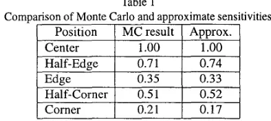
Table 1

Comparison of Monte Carlo and approximate sensitivities Position

1

MCresult

1

Approx. Center

I

1.00

I

1

.oo

-

Half-Corner

1

0.51

I

0.52

Comer

I

0.21

I

0.17

As noted above, straight-forward computation of the weights t i j would require the computation of integrals over three positions and an energy variable for each gamma and yield a total of N’N, results. We use here an approach requiring computation of just

N, back-projections with just

2 N N , stored results. The approximation of t i j is done in a three part fashion. We begin with our original model in which the weights are computed for only those pixels which are intersected by the back-projected cone of each measurement

i.

As we seek to compute the relative values of the weights (from equation 1 we see that the iteration is independent of any normalization on the tij), we note that we require 2 factors.

The first to describe the relative probabilities between the measurements

i,

and the second to describe the probabilities within the measurements, i. e., the relative probability that the gamma giving rise to the measurement

i

was emitted from pixel j.

We assume that the first factor is influenced primarily by the relative differential cross section and the escape probability of the scattered photon in the first detector:

[image:2.619.379.491.87.208.2] [image:2.619.333.530.372.460.2]

I13

where ut is the total cross section at the scattered photon energy in the first detector, 2 1 2 the distance traveled through the first detector along the ray between the first and second collisions, and

%

the differential Compton cross section. Since we need only to determine functional dependence and not absolute values, we approximate $$ as the Klein-Nishina cross section at the given energy divided by the square of the distance between the two collisions.

The second factor, the relative probabilities that a given event originated from a gamma emitted from the various pixels, must take into account the pixel sensitivities sj as well as the resolution loss brought on by Doppler broadening and the finite resolution in the energy measurement. We use the approximate relative sj's of equation 3 for the first factor here, and then assume that the other effects are described by the angular resolution of back-projected cones determined for

a given system [5, 71. We assume that the value of the full width at half maximum of the cone-spread function is constant for all possible Compton scattered energies for a given initial energy, which is valid over most of the angular spectra in which Compton cameras are designed to function [SI. We then assume that the cone spread distribution, which is not Gaussian because of the long Doppler tails, can be modeled by adding to

.9 times a Gaussian about the computed standard deviation to

10% of a Gaussian distribution with 3 times the cone spread standard deviation,

where T is the normal distance in the image plane from the

pixel to the back-projected cone. The relative value assigned to each pixel would be the integral of this function over the area of the pixel. As we plan to store for each gamma only a list of intersected pixels and to generate the pixel weights of all neighboring pixels at each iteration step, we seek to approximate these integrals. If we assume the conics to be linear within a given pixel and have T

< <

U (this corresponds to

pixel dimension

L

less than the cone spread in the image plane), it can be shown that integrals over pixels which are intersected by conics vary in the range from 2

-

L2/8u2 to 2

-

3L2/4a2

depending upon the orientation of the conics and the normal distance to the center of the pixel. For practical applications,

L 2 / n 2 will be less than 0.1, and we can take the integrals to be constant. We therefore have that the relative weight of a

non-intersected, neighboring pixel j in the computation of t i j for a given

i

is dependent solely on the distance between it and a pixel of intersection. Neighbors are chosen by taking them along either rows or columns of the image space (depending if the conic intersected the image space in a more vertical or horizontal orientation respectively), so the distance to the mth neighbor is mL, and the relative weight of that pixel is taken as

f(m) cc . g e x p ( - ( m ~ ) ~ / 2 u ~ >

+

. l e x p ( - ( m ~ ) ~ / 2 ( 3 c r ) ' ) . (6) Since the selection of which neighboring pixels to include is made normal to the conic, even though the integral over the spread function in the pixels is fairly independent of the orientation of the conic, for conics which intersect the image

space with slopes not near to zero or to infinity, the distances to the center of the neighbor pixels are smaller than L , and the relative weight for the mth neighbor taken from equation 6 needs to be adjusted. We do this by multiplying f ( m ) by a

relative correction which is a maximum of 1 for slopes of 1

(which correspond to minimum distances between intersected pixel centers and neighbor centers) and is given by:

(7)

Here s is a factor related to the slope of a conic with the given cone cosine X and axis direction given by u z i f u y j

+

u z k . We approximate the slope of the conic by translating the focus from

( a z 1 a y ] a,) to

(x',

Y',

2')

=

(x-,,

vy,

2 4 , ) where (z, y,

z )

is the pixel center, and using

The slope parameter s is then given by c ~ s ~ [ t a n - ~ ( $ ) ] if

) d y / d z ] is less than 1, and sin2[tan-'( $)] otherwise. To summarize the procedure, the t i j are computed by first determining a list of pixels intersected by the back-projected conic for each gamma, as described in [ 5 ] . Next, the relative probability between the measurements f(i) is computed according to equation 4. At each step of the iteration, the weights are approximated by branching out either vertically or horizontally from the intersected pixels and multiplying

f(

i)

first by the sensitivity s j , then by the pre-computed spread function f(m), and finally by the slope dependent correction fm(s) for each of the m neighbors in both the plus and minus direction. Storage requirements are minimized to 1 real number per intersected pixel by adding the real value of f ( m ) (which is always less than 1) to the integer pixel ID number, and using the sign of the value to indicate if the branch is horizontal or vertical. Thus we save a factor of N / 2 in storage at the expense of taking an absolute value and doing an real to integer conversion, plus 3 extra multiplications per particle per pixel at each iteration step. For the current work, in which only workstations with 256MB or less of memory were available, this allows us to model 500,000 particles on a 64x64 image grid without exhausting memory.

As with the assumptions made in determining an expression for the sensitivities, the approximations described above will hold best for normally incident gammas, and will be most accurate for high angle scatters and for the pixels along the back-projections. Small scattering angles yield greater curvature in the back-projections (which are approximated above as straight lines), and acute angles of incidence introduce more variation in the image to detector distances between the pixels near and far from the back-projections. This introduces some error in both the solid angle computation and the cone-spread FWHM.

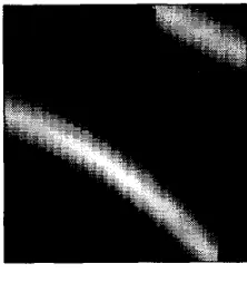
Figures 2 and 3 show the back-projection for a single particle

the model here are evident from the discontinuities in the back- projection. Note from the figure that for this conic, neighbors were chosen in the vertical direction.

back-projections with large variations in the first derivatives of the conics in the image space. For such particles, in which the slope changes from near zero to near infinity, either the nearly horizontal or the nearly vertical portion will be mis-modeled.

111.

RESULTS

AND

DISCUSSION

[image:4.619.129.240.122.241.2]

Results are given below for reconstructions using the current method on measured data for several source configurations. The experimental data taken with the prototype C-SPRINT detector [ 101 described earlier. Reconstructed images of a point source, using a 15 cm FOV and a 64x64 grid are shown below at iterations 0, 50, and 100. Computations were performed on a Ultra 10 workstation, and required approximately 1 minute per iteration using 100,000 particles.

Fig. 2 Computed back-projections of representative particles . .

[image:4.619.372.492.268.390.2]

0 0

Fig. 5 Reconstructed point source, 0th iteration

[image:4.619.130.241.298.425.2]

Fig. 3 Approximate back-projections of representative particles

Figure 4 shows cross sectional cuts through the image plane of the weights for the approximate method (solid lines) and the detailed computation (crosses) for two sets of back projections, the first with slope very nearly normal to the image space, and the second with slope close to

45

degrees. The rigorous and approximate models agree well for both cases, except quite far out on the Doppler tails.

Fig. 4 Computed cross sectional back-projections of representative particles

The obvious weakness of the present method, which relies on several linearity approximations, will be for image spaces with large pixel dimensions relative to Doppler spread, and for particles with very small scattering angles, leading to

0 0

Fig. 6 Reconstructed point source, 50th iteration

The Oth is simply the back-projection, and figures 6 and 7 clearly show the image reducing to the expected point source at the center of the image field. The full width at half maximum of the point spread of the image was determined to be roughly

8 mm (see figure 8). From measurements of the point spread of the image at higher interations, it was seen that convergence of the algorithm was not achieved in 100 iterations. No systematic analytic criteria for determing convergence was applied.

[image:4.619.372.492.431.563.2] [image:4.619.130.245.548.631.2]

115

[image:5.616.358.483.75.200.2]

0 0

Fig. 7 Reconstructed point source, 100th iteration

x

10-

10

8

6

4

2

0

0

20

40

Fig. 8 Profile of reconstructed point source, 100th iteration

between the parallel sections was 6 cm, and the intensity of the angled line 1/2 that of the parallel lines. The inherent device

FWHM cone spread at the 11 cm source to detector distance was computed to be 1.5 cm [8], and results are shown here for reconstructions after 100 iterations using m of 0, 8, and 16

pixels on either side of the initial back-projected cones (for the m

=

0 case

,

as the higher iteration images are extremely noisy, the 20th iteration is shown). [image:5.616.125.238.78.208.2]

We see that there is no discernible improvement in the images quality from treating more of the tails of the cone spread. This would indicate that the errors in the computation of the sensitivities and the weights for pixels near to the back-projection have a greater impact on the performance of the algorithm than the truncation of the weights at larger distances, and suggests that future effort be devoted to eliminating the approximations involved in determining t ; j . Candidate targets enhancements are the use of spatially varying cone spread FWHM, correcting for escape probabilities and solid angle effects for the scattered photons, and more accurately approximating the cone-spread for pixels adjacent to the back-projection, accounting for both non-normal angle of incidence and position and curvature of the back-projected cone.

Fig. 9 Reconstructed line phantom using only central pixel, 20th iteration

Fig. 10 Reconstructed line phantom using 8 nearest pixels, 100th iteration

IV. CONCLUSIONS

A computationally efficient method has been devised for determining the relative sensitivities and system matrix coefficients for Compton scatter cameras with planar first detectors. The method has been shown to give results with excellent agreement in comparison to both Monte Carlo and rigorous analytical results. Images have been reconstructed from experimental data for point and extended sources.

V.

REFERENCES

[l] T. Hebert, R. Leahy, M. Singh, “Three-dimensional maximum- likelihood reconstruction for an electronically collimated single- photon-emission imaging system,” J. Opt. Soc. Am., vol. 7, 1990 [2] H.H. Barrett, T. White, and L.C. Parra, “List-mode likelihood,”

J.

Opt. Soc. Am., vol. 14, 1997pp. 2914-2923.

[3] L.C. P a m and H.H. Barrett, “List-mode likelihood: EM algorithm and image quality estimation demonstrated on 2-D PET,” IEEE Trans. Med. Imag., vol. 17, 1998 pp. 228-235.

[image:5.616.118.243.270.414.2] [image:5.616.356.484.272.390.2]

[image:6.612.126.237.75.196.2]

Fig. 11 Reconstructed line phantom using 16 nearest pixels, 100th iteration

scatter cameras,” IEEE Trans. Nucl. Sci., vol. 44, 1997 pp. 250-

254.

S.J. Wilderman, “Vectorized algorithms for the Monte Carlo simulation of kilovolt electron and photon transport,” University of Michigan, Ann Arbol; Ml, Ph. D. dissertation, 1990. J.W. LeBlanc, N.H. Clinthome, C-h. Hua, E. Nygard, W.L. Rogers, D.K. Wehe, P. Weilhammer, S.J. Wilderman, “C-Sprint: A prototype Compton camera system for low energy gamma ray imaging”, presented at IEEE Nucl. Sci. Sym. and Med. Imaging Con$, Albuquerque, N.M., 1997.

J.W. LeBlanc, “A Compton Camera for Low Energy Gamma Ray Imaging in Nuclear Medicine Applications,” University of Michigan, Ann Arbor, MI, Ph. D. dissertation, 1999.

T. Kragh, private communication, Oct 1999.

J.W. LeBlanc, X. Bai, N.H. Clinthome, C-h. Hua, D. Meier, W.L. Rogers, D.K. Wehe, P. Weilhammer, S.J. Wilderman, “99mT~ Imaging Performance of the C-SPRINT Compton Camera,” presented at IEEE Nucl. Sci. Sym. and Med. Imaging