R E S E A R C H
Open Access
Adaptive group bridge estimation for
high-dimensional partially linear models
Xiuli Wang and Mingqiu Wang
**Correspondence: [email protected] School of Statistics, Qufu Normal University, Jingxuan West Road, Qufu, 273165, P.R. China
Abstract
This paper studies group selection for the partially linear model with a diverging number of parameters. We propose an adaptive group bridge method and study the consistency, convergence rate and asymptotic distribution of the global adaptive group bridge estimator under regularity conditions. Simulation studies and a real example show the finite sample performance of our method.
MSC: 62E20; 62J07; 62F12
Keywords: adaptive group bridge; high dimension; partially linear model
1 Introduction
Consider the following model:
Y= xTβ+f(U) +ε, ()
where x = (xT
,xT, . . . ,xTpn)
Tis a covariate vector withx
j= (Xjk,k= , . . . ,dj)Tbeing adj× vector corresponding to thejth group in the linear part,β= (βTj,j= , . . . ,pn)T withβj being thedj× vector of regression coefficients,f is an unknown function ofU, and εis the random error with mean zero. Without loss of generality,U is scaled to [, ]. Furthermore, (x,U) andεare independent.
Variable selection for high-dimensional data is a hot and important issue. Penalized regression methods have been widely used in the literature such as [–], and so on. Among these methods, bridge regression including lasso and ridge as two well-known special cases has been studied by many authors (e.g., [–]). [] studied adaptive bridge estimation for high-dimensional linear models. In addition, group structure of variables arise always in many contemporary statistical modeling problems. [] proposed a group bridge method which not only effectively removes unimportant groups, but also maintains the flexibility of selecting variables within identified groups. [] investigated an adaptive choice of the penalty order in group bridge regression.
The aforementioned model () is just the partially linear model that originated from []. The partially linear model is a common semiparametric model enjoying the inter-pretability and flexibility. Our contributions in this paper include: () we propose an adap-tive group bridge method to achieve the group selection for a high-dimensional partially linear model; () we consider the choice of indexγ in the adaptive group bridge and use
leave-one-observation-out cross-validation (CV) to implement this choice. It can signif-icantly reduce the computational burden; () we give the consistency, convergence rate and asymptotic distribution of the adaptive group bridge estimator which is the global minimizer of the objective function.
The rest of the article is organized as follows. Section gives the adaptive group bridge method. In Section , we show the assumptions and asymptotic results for the global adap-tive group bridge estimator. Section shows computational algorithm and selection of tuning parameters. Simulation studies and real data are presented in Section . Section gives a short discussion. Technical proofs are relegated to Appendix.
2 Adaptive group bridge in the partially linear model
Suppose that we have a collection of independent observations{(xi,Ui,Yi), ≤i≤n}from model (). That is,
Yi= xTiβ+f(Ui) +εi, i= , . . . ,n, ()
whereε, . . . ,εnare i.i.d. random errors with mean zero and finite varianceσ<∞. To obtain an estimate of functionf(·), we employ a B-spline basis. DenoteSnas the space of polynomial splines of degreem≥. Let{Bk(u), ≤k≤qn}be a normalized B-spline basis withBk∞≤, where · ∞is the sup norm. Then, for anyfn∈Sn, we have
fn(u) = qn
j=
Bj(u)αjB(u)Tα.
Under some smoothness conditions, the nonparametric functionf can well be approxi-mated by functions inSn.
Consider the following adaptive group bridge penalized objective function:
n
i=
Yi– xTi β– B(Ui)Tα
+ pn
j=
λjβjγ, ()
where λj, j= , . . . ,pn, are the tuning parameters, and · denotes the L norm on
the Euclidean space. Let Y = (Y, . . . ,Yn)T, X= (Xijk, ≤i≤n, ≤j≤pn, ≤k≤dj) =
(x, . . . , xn)Tand Z = (B(U), . . . , B(Un))T. Then () can be changed into
Ln(β,α) =Y–Xβ– Zα+ pn
j=
λjβjγ. ()
For someβ, the optimalαminimizingLn(·) meets the partial differential equation
∂Ln(β,α)/∂α= ,
namely,
LetH= Z(ZTZ)–ZT, note thatHis a projection matrix. We can rewrite the expression () as follows:
Qn(β) =(I–H)(Y –Xβ)
+ pn
j=
λjβjγ. ()
For some fixedγ > , defineβˆ=arg minQn(β), thenβˆ is called the adaptive group bridge estimator. Ifβˆ is obtained, then the estimatorαˆ can be achieved. Thus we can get the estimator of the nonparametric part, namely,ˆfn(u) = B(u)Tα.ˆ
3 Asymptotic properties
In this section, we show the oracle property of the parametric part. For convenience of the statement, we first give some notations. Define g(u) =E(x|U=u) andx˜= x –E(x|U). Let(u) be the conditional covariance matrix ofx˜, i.e.,(u) =cov(x˜|U=u). Denote as the unconditional covariance matrix ofx˜, i.e., =E[(U)]. The corresponding sample version is G = (g(U), . . . , g(Un))Twith g(Ui) =E(xi|Ui) andX= (x˜, . . . ,x˜n)Twithx˜i= xi– E(xi|Ui).
Let the true parameter be β= (βT, . . . ,βTpn)T (βT
,βT)T. Let A={≤j≤pn : βj = }be the index set of the nonzero groups. Without loss of generality, we assume that coefficients of the firstkngroup are nonzero, i.e.,A={, , . . . ,kn}. Let|A|=knbe the cardinality of the setA, which is allowed to increase withn. Forj∈/A,βj= . De-fineβ= (βTj,j∈A)T,β
= (βTj,j∈/A)T. Letd∗=max≤j≤pndj,ϕn=max{λj,j∈A}and ϕn=min{λj,j∈/A}.
Corresponding to the partition ofβ, denoteβˆ= (βˆT(),βˆT())Tand decompose
X= (XX), G= (GG), X= (XX), =
.
The following conditions are required for the B-spline approximation of functionf.
(C) The distribution ofUis absolutely continuous, and its density is bounded away
fromand∞.
(C) (Hölder conditions off(·)andgj(·), wheregjis thejth component ofg) Letl,δand Mbe real constants such that <δ≤andM> .f(·)andgj(·)belong to a class of functionsH,
H= h:h(l)(u) –h(l)(u)≤M|u–u|δ,for≤u,u≤
,
where <l≤m– andr=l+δ.
The following part lists all the reasonable conditions which are necessary to attain the asymptotic results.
(A) Letλmax( )andλmin( )be the largest and smallest eigenvalue of , respectively.
There exist constantsτandτsuch that
(A) There exist constants <b<b<∞such that
b≤min βj, ≤j≤kn
≤max βj, ≤j≤kn
≤b.
(A) n–XT(I–H)X– →P ;E[tr(XT(I–H)X)] =O(npn).
(A) d∗=O(),pn/n→andn–ϕnkn→.
(A) (a)ϕnkn//( √
npn+n√pnqn–r)→; (b)ϕn(
n–p
n+√pnq–nr)γ–/n→ ∞.
(A) For every≤j≤pnand≤k≤dj,E[Xjk–E(Xjk|U)]is bounded. Furthermore,
E(ε)is bounded.
Conditions (A) and (A) are commonly used. Condition (A) holds under some condi-tions. The proof can be found in Lemmas and in []. Condition (A) is used to obtain the consistency of the estimator. Condition (A) is needed in the proof of convergence rate. Condition (A) is necessary to attain the asymptotic distribution.
Theorem .(Consistency) Suppose thatγ > and conditions(A)-(A)hold,then
ˆβ–β=OP
n–d∗pn+qn–r+n–ϕnkn
,
namely, ˆβ–β→P .
Theorem . implies that under some conditions the estimators converge to the true values of parameters.
Theorem .(Convergence rate) Suppose that conditions(A)-(A)hold,then
ˆβ–β=OP
n–p
n+√pnq–nr
.
This theorem shows that the adaptive group bridge can give the optimal convergence rate withpn→ ∞.
Theorem .(Oracle property) Suppose that <γ < ,n–k
nqn→and nq–n r→.If conditions(A)-(A)are satisfied,then we have
(i) Pr(βˆ()= )→,n→ ∞; (ii) Letu
n=nωTn(XT(I–H)X)– (XT(I–H)X)–ωnwithωnbeing some kn
j=dj-vector withωn= ,then
n/u–n ωTn(βˆ()–β)→D N,σ.
This theorem states that the adaptive group bridge performs as well as the oracle [].
4 Computational algorithm and selection of tuning parameters
4.1 Computational algorithm
We take the initial valueβ(). Here the ordinary least square estimate is chosen as the initial valueβ(). The penalty termpλj(βj) =λjβjγ can be approximated as
pλj
βj≈pλjβ
()
j + p
λjβ
()
j /β
()
j βj–β
()
j
,
whenβ()j > . The following iterative expression ofβcan be obtained:
β()=XT(I–H)X+n
λ,γ
β()–XT(I–H)Y, ()
where
λ,γ
β()=diag
p λj(β
()
j )
β()j Idj,j= , . . . ,pn
,
withIdjbeing adj×djunit matrix. If someβ
()
j is smaller than –, then we setβ
()
j = . The finial estimate can be obtained iteratively by formula () until the convergence is achieved.
4.2 Selection of the tuning parameters
For our method,qn,γ, andλj(j= , . . . ,pn) should be chosen. For convenience, cubic spline basis (m= ) is used. We setqn= . Simulation results demonstrate that this choice per-forms quite well. There are also many tuning parameters that should be chosen. In fact, we only need to select one tuning parameter by settingλj=λ/β()j . We use ‘leave-one-observation-out’ cross-validation (CV) to selectλandγ. Due to the convergence of the algorithm, we have
ˆ
β=XT(I–H)X+nλ,γ(β)ˆ
–XT(I–H)Y,
whereβˆ is obtained based on the whole data set. Note that it is the solution of the ridge regression
Y∗–X∗β+nβTλ,γ(β)β,ˆ ()
where Y∗= (I–H)Y andX∗= (I–H)X. Let Y∗= (y∗, . . . ,y∗n)TandX∗= (x∗
, . . . , x∗n)T. The CV error is
CV(λ,γ) = n
n
i=
y∗i – x∗iTβˆ–i,
whereβˆ–iis achieved by solving () without theith observation. The computation of the CV error is intensive, so we will use the following formula, which can be proved similar to []:
CV(λ,γ) = n
n
i=
where Dii is the (i,i)th diagonal element of (I–H)X[XT(I–H)X+nλ,γ(β)]ˆ –XT(I–
H). It is obvious that this method can significantly reduce the computational bur-den.
5 Simulation studies and application
In this section, we investigate the finite sample performance of the adaptive group bridge method through simulations and a real data application.
5.1 Monte Carlo simulations
We simulate datasets consisting ofnobservations from the following partially linear model:
Yi= pn
j=
xTijβj+cos(πUi) +εi, i= , . . . ,n,
wheren= , and the errorεi∼N(,σ) withσ= ., , . We consider that there are pngroups withpn= , , and each group consists of three variables. The true values of parametersβT = (., , .),βT = (, –, ),βT = (., ., .),βT=· · ·=βTpn= (, , ). Uifollows the uniform distribution on [, ]. To generate covariate x = (xT,xT, . . . ,xTpn)
T
withxj= (Xjk,k= , , )T, we first simulateR, . . . ,Rpn independently from the standard
normal distribution. Next, simulateZj,j= , . . . ,pn, from a multivariate normal distribu-tion with the mean zero andCov(Zj,Zl) = .|j–l|. Then the covariates are generated as Xjk= (Zj+R(j–)+k)/
√
,j= , . . . ,pn,k= , , .
We compare the adaptive group bridge (AGB) with the group lasso (GL) and the group bridge (GB). The following three performance measures are calculated:
. Lloss of parametric estimate, which is defined asβ–β. . Average number of nonzero groups identified by the method (NN).
. Average number of nonzero groups identified by the method that are truly nonzero (NNT).
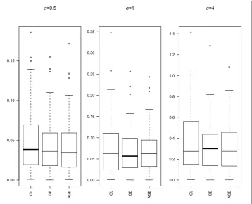
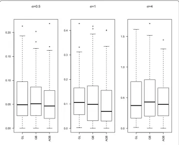
Group selection results are depicted in Table . The numbers in the parentheses in the columns labeled ‘NN’ and ‘NNT’ are the corresponding sample standard deviations based on the runs. Boxplots of theLlosses under different settings are given in Figures -.
From Table , we can have the following observations:
() Both GB and AGB perform better than GL for all settings. All these three methods can retain all the true nonzero groups, but GL always keeps more redundant groups that are unrelated with the response than both GB and AGB.
() AGB performs much better for largerσandpn. Whenpn= for AGB, groups
selected for the caseσ= are about .% lower than that for the caseσ= .. While groups selected for GB decrease by .% in the same situation.
() Forpn= , GB performs better than AGB, but the stability of GB is bad forσ= . Figures - presentLlosses with varyingσ andpn. We can see that the performances
of estimates are similar for GB and AGB. Forpn= and , both GB and AGB perform better than GL. However, when pn= , the median ofLlosses for all these three are
Table 1 Group selection results
pn Method σ= 0.5 σ= 1 σ= 4
NN NNT NN NNT NN NNT
10 GL 7.80 3 7.59 3 6.02 3
(1.231) (0) (2.396) (0) (1.255) (0)
GB 4.64 3 4.80 3 4.55 3
(1.259) (0) (1.356) (0) (1.258) (0)
AGB 5.22 3 5.00 3 4.56 3
(1.605) (0) (1.735) (0) (1.131) (0)
30 GL 20.47 3 11.49 3 14.46 3
(2.504) (0) (4.464) (0) (2.022) (0)
GB 11.04 3 10.96 3 10.18 3
(3.643) (0) (3.784) (0) (2.350) (0)
AGB 13.06 3 10.64 3 9.57 3
(5.510) (0) (5.921) (0) (2.046) (0)
50 GL 33.17 3 16.48 3 22.37 3
(3.223) (0) (5.018) (0) (3.308) (0)
GB 17.23 3 17.79 3 15.96 3
(4.608) (0) (3.952) (0) (3.284) (0)
AGB 19.25 3 15.67 3 15.68 3
(8.437) (0) (8.385) (0) (3.684) (0)
[image:7.595.119.478.395.685.2]Figure 2 Boxplots ofL2loss forpn= 30.
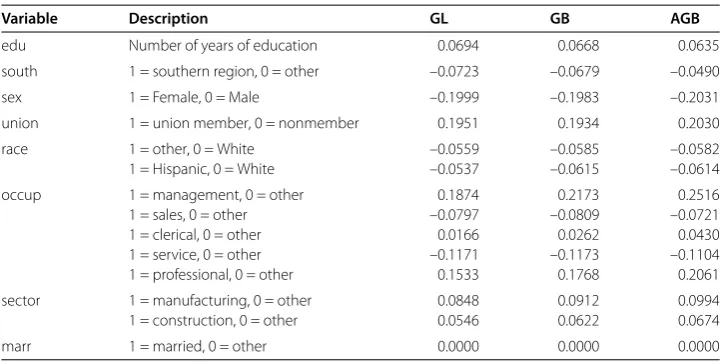
Table 2 Estimates of the wage data
Variable Description GL GB AGB
edu Number of years of education 0.0694 0.0668 0.0635
south 1 = southern region, 0 = other –0.0723 –0.0679 –0.0490
sex 1 = Female, 0 = Male –0.1999 –0.1983 –0.2031
union 1 = union member, 0 = nonmember 0.1951 0.1934 0.2030
race 1 = other, 0 = White –0.0559 –0.0585 –0.0582
1 = Hispanic, 0 = White –0.0537 –0.0615 –0.0614
occup 1 = management, 0 = other 0.1874 0.2173 0.2516
1 = sales, 0 = other –0.0797 –0.0809 –0.0721
1 = clerical, 0 = other 0.0166 0.0262 0.0430
1 = service, 0 = other –0.1171 –0.1173 –0.1104
1 = professional, 0 = other 0.1533 0.1768 0.2061
sector 1 = manufacturing, 0 = other 0.0848 0.0912 0.0994
1 = construction, 0 = other 0.0546 0.0622 0.0674
marr 1 = married, 0 = other 0.0000 0.0000 0.0000
5.2 Wage data analysis
The workers’ wage data from Berndt[] contains a random sample of observations on variables sampled from the current population survey of . It provides information on wages and other characteristics of the workers, including continuous variables: the number of years of education, years of work experience, age and nominal variables: race, sex, region of residence, occupational status, sector, marital status and union membership. Our goal is to study the important factors for the wage, so it is reasonable to use our proposed method for these data.
From the residual plot, we can easily see that the variance of wages is not a constant. So thelogtransformation is used to stabilize the variance of wages. Due to the multicollinear-ity problem between age and experience, we need to get rid of either age or experience. Here we remove the age variable from the model. Xie and Huang [] analyzed these data without considering the transformation ofY. Furthermore, they did not consider group selection of factors. Similar to Xie and Huang [], we fit these data using a partially linear model withUbeing ‘years of work experience’.
Table reports estimated regression coefficients of GL, GB and AGB. All these three methods exclude marital status. We use the first observations as a training dataset to select and fit the model, and use the rest of observations as a testing dataset to evalu-ate the prediction ability of the selected model. The prediction performance is measured by the median of{|yi–yˆi|,i= , , . . . , }for GL, GB and AGB using the testing data, respectively. Hereyi’s are those observations in the testing dataset andyˆi’s are corre-sponding prediction values. The median absolute prediction errors of GL, GB and AGB are ., . and ., respectively. Therefore, we can conclude that the AGB gives the smallest prediction error, so it is an attractive technique in group selection.
6 Discussion
Appendix
Proof of Theorem. By the definition ofβ, it is easy to getˆ
(I–H)(Y –Xβ)ˆ + pn
j=
λj ˆβjγ≤(I–H)(Y –Xβ)
+ pn
j=
λjβjγ,
that is,
(I–H)(Y –Xβ)ˆ –(I–H)(Y –Xβ)≤ pn
j=
λjβjγ.
As Y =Xβ+f(U) +εwithf(U) = (f(U), . . . ,f(Un))Tandε= (ε, . . . ,εn)T, we can rewrite
the upper inequality as follows:
(I–H)X(βˆ–β)– f(U) +εT(I–H)X(βˆ–β)≤ pn
j=
λjβj
γ
.
Let
an=n–/
XT(I–H)X/(βˆ–β
),
bn=n–/
XT(I–H)X–/XT(I–H)f(U) +ε.
Then we have
an≤
an–bn+bn
≤ n
pn
j=
λjβjγ+ bn.
Since|A|=kn, under condition (A),
n
pn
j=
λjβjγ =O
ϕnkn n
.
While
bn= n
f(U) +εT(I–H)XXT(I–H)X–XT(I–H)f(U) +ε
≤ nε
TAε+ nf(U)
TAf(U), ()
where
A= (I–H)XXT(I–H)X–XT(I–H).
For the first term on the right-hand side of (),
E
nε
TAε
=σ
n tr
Thus
n–εTAε=OP
n–d∗pn
. ()
For the second term on the right-hand side of (), by conditions (C) and (C),
E
nf(U)
TAf(U)
≤
nE λmax (I–H)X
XT(I–H)X–
XT(I–H)
×trf(U)T(I–H)f(U)
= nE
f(U)T(I–H)f(U)=Oqn–r. ()
Combining ()-(),
bn=OP
n–d∗pn+q–n r
.
By conditions (A) and (A),
Ean= nE
(βˆ–β)TXT(I–H)X(βˆ–β)
=E
(βˆ–β)T
nX
T(I–H)X–
(βˆ–β)
+E(βˆ–β)T (βˆ–β)
≥ τ
E ˆβ–β
.
Therefore
ˆβ–β=OP
n–d∗pn+qn–r+n–ϕnkn
.
Under condition (A), we have
ˆβ–β→P .
Proof of Theorem . Letμn=n–p
n+q–nr +
n–ϕn
kn, we can choose a sequence
{rn,rn> }which satisfiesrn→. PartitionR
pn
j=dj\{}into shells{S
nj:j= , , . . .}, where Snj={β: j–rn≤ β–β< jrn}. For an arbitrary fixed constantL∈R+, if ˆβ–βis
larger than Lrn,βˆis in one of the shells withj≥L, we have
Pr ˆβ–β ≥Lrn
=
l>L,lr n>Lμn
Pr(βˆ∈Snl)
+
l>L,lrn≤Lμn
Pr(βˆ ∈Snl) (Lis an arbitrary constant),
where
l>L,lrn>Lμ n
Pr(βˆ∈Snl)≤Pr ˆβ–β ≥L–μ
n
and
l>L,lr n≤Lμn
Pr(βˆ∈Snl)
=
l>L,lrn≤Lμn
Pr
ˆ
β∈Snl,n ≤ τ
+
l>L,lr n≤Lμn
Pr
ˆ
β∈Snl,n> τ
,
wheren=n–XT(I–H)X– . By condition (A),
l>L,lr n≤Lμn
Pr
ˆ
β∈Snl,n>τ
≤Pr
n>τ
=o().
Therefore,
Pr ˆβ–β ≥Lrn
=o() +
l>L,lrn≤Lμn
Pr
inf
β∈Snl
Qn(β) –Qn(β)
< ,n ≤ τ
.
Since
Qn(β) –Qn(β)
=(I–H)X(β–β)– f(U) +εT(I–H)X(β–β)
+ pn j= λj
βjγ–βjγ
≥(I–H)X(β–β)– f(U) +εT(I–H)X(β–β)
+ kn j= λj
βjγ–β jγ
= In+ In+ In.
For In,
In≥ inf
β∈Snl
nτ
β–β
,
for allβ∈Snl, there existsβ–β≥l–rn, therefore In≥nτl–rn. For In, we have
|In|=
kn
j=
λjγβ∗j
γ–
βj–βj
≤ϕnγ
kn j= β∗ j γ–
whereβ∗j is betweenβjandβj. By condition (A) and since we only need to considerβ withβ∈Snl, lrn≤Lμn, there exists a constantC> such that
|In| ≤Cϕnγ
kn
j=
βj–βj ≤Cϕnkn/γβ–β.
So for allβ∈Snlsuch that|In| ≤Cϕnkn/γlrn, by the Markov inequality, we have
Pr
inf
β∈Snl
Qn(β) –Qn(β)
≤
≤Pr
sup
β∈Snl
|In| ≥nτl–rn–Cϕnkn/γlrn
≤ E(supβ∈Snl|In|)
nτl–rn–Cϕnkn/γlrn .
Using the Cauchy-Schwarz inequality, we have
E
sup
β∈Snl
|In|
≤Ef(U) +εT(I–H)XXT(I–H)f(U) +ε/
×E
sup
β∈Snl
β–β /
≤l+/rn
EεT(I–H)XXT(I–H)ε
+Ef(U)T(I–H)XXT(I–H)f(U)/,
where
EεT(I–H)XXT(I–H)ε=σEtr(I–H)XXT(I–H)=O(np n)
and
Ef(U)T(I–H)XXT(I–H)f(U)
≤EtrXT(I–H)Xtrf(U)T(I–H)f(U)
=O(npn)O
nq–n r=Onpnq–n r
.
Accordingly,
E
sup
β∈Snl
|In|
≤Clrn √
npn+n√pnq–nr
.
Then we can get
l>L,lrn≤Lμ n
Pr(βˆ∈Snl)≤ l>L
Clrn(√npn+n√pnq–nr) nτl–rn–Cϕnkn/γlrn
We choosern= (√pn/n+√pnq–nr), we have
l>L,lrn≤Lμn
Pr(βˆ∈Snl) =
l>L
C
τl––Cϕnkn/γ/( √
npn+n√pnq–nr) .
By condition (A)(a)ϕnkn//( √
npn+n√pnq–nr)→, for sufficiently largen,
l––Cτ–λjkn// √
npn+n√pnM
–rg
n
≥l–.
Thus
l>L,lrn≤Lμ n
Pr(βˆ∈Snl)≤ l>L
C
l– ≤C –(L–).
LetL→ ∞, then
l>L,lrn≤Lμn
Pr(βˆ∈Snl)→.
Hence
ˆβ–β=OP
n–p
n+√pnq–nr
.
Proof of Theorem. (i) By Theorem ., for sufficiently largeC,βˆ lies in the ball{β:
β–β ≤vnC}with probability converging to , wherevn=
n–p
n+√pnq–nr. Letβ()=
β+vnνandβ()=β+vnν=vnνwithν=ν+ν≤C. Let
Vn(ν,ν) =Qn(β(),β()) –Qn(β, ) =Qn(β+vnν,vnν) –Qn(β, ).
Then βˆ andβˆ can be attained by minimizingVn(ν,ν) over ν ≤C, except on an
event with probability converging to zero. We only need to show that, for someνandν
withν ≤C, ifν> ,
PrVn(ν,ν) –Vn(ν, ) >
→, n→ ∞.
Some simple calculations show that
Vn(ν,ν) –Vn(ν, ) =vn(I–H)Xν
+ vn(Xν)T(I–H)(Xν)
– vn
f(U) +εT(I–H)(Xν) +
j∈/A
λjvnνjγ
= IIn+ IIn+ IIn+ IIn.
For the first two terms IInand IIn,
IIn+ IIn≥–vn(I–H)Xν
= –nvnCoP() +τ
For IIn, we have
Ef(U) +εT(I–H)Xν
≤ Ef(U)T(I–H)XννTXT(I–H)f(U)
+εT(I–H)XννTXT(I–H)ε
≤C E
trXT(I–H)X
trf(U)T(I–H)f(U)
+σEtrXT(I–H)X
=Onpnq–nr+npn
.
Thus we have
IIn=vn
np/n q–nr+n/p/n OP().
For IIn, by <γ< ,
j∈/A
vnνjγ /γ
≥
j∈/A
vnνj /
=vnν.
Accordingly,
IIn≥ϕnvγnνγ.
By condition (A)(b), for someν> , we have
PrVn(ν,ν) –Vn(ν, ) >
→.
(ii) Letωnbe some kn
j=dj-vector withωn= . By Theorem .(i), with probability tending to , we have the following result:
∂Qn(β())
∂β()
β()=βˆ()
=XT(I–H)X(βˆ()–β) –XT(I–H)
f(U) +ε+ξn= ,
whereξn= (λγ ˆβγ–βˆ
T
, . . . ,λknγ ˆβkn
γ–βˆT
kn)
T. We consider the limit distribution
n–/ωTn –/ XT(I–H)X
(βˆ()–β)
=n–/ωTn –/ XT(I–H)f(U) +n–/ωTn –/ XT(I–H)ε
–n–/ωTn –/ ξn
=Jn+Jn+Jn.
ForJn,
Jn=n–ωTn –/ XT(I–H)f(U)=OP
ForJn, by conditions (A) and (A), we have
EJn≤n–τ–ϕnγ
kn
j=
E ˆβj(γ–)=On–ϕnkn
.
ForJn,
Jn=n–/ωTn –/ GT(I–H)ε+n–/ωTn –/ XTε
–n–/ωTn –/ XTHε
=Kn+Kn+Kn.
Under conditions (C) and (C),
EKn=n–ωTn –/ EGT(I–H)εεT(I–H)G
–/
ωn
=Oknq–n r
.
By condition (A), we have
EKn=n–ωTn –/ EXTHεεTHX
–/
ωn
=On–knqn
.
Now we focus onKn
Kn=n–/ωTn –/ XTε
=√ n
n
i=
sniεi.
First,
E(sniεi) = ;
Var
n
i=
sniεi
= n
i=
Var(sniεi) =σ.
Next we verify the conditions of the Lindeberg-Feller central limit. For any> ,
n
i=
Esniεi|sniεi|>
=nEsnε|snε|>
≤nEsnε/Pr|snε|>
/
.
By condition (A),
Esnε=n–E ωTn –/ x–E(x|U)
x–E(x|U)
T –/
ωn
Eε
≤n–ρminωnωTn
ρmax –E x–E(x|U)
T
x–E(x|U)
≤n–ρminωnωTn
ρmax –Eεknd∗ kn
j=
dj
k=
EXjk–E(Xjk|U)
=Oknn–
and
P|snε|>
≤
E(snε)
= σ
n –ωT
n –/ E x–E(x|U)
x–E(x|U)
T –/
ωn
= σ
n
–=On–.
Thus we have
n
i=
Esniεi|sniεi|>
=Onknn–n–/
=o().
This means thatKn
D
→N(,σ). Using Slutsky’s theorem, we have
n–/ωTn –/ XT(I–H)X
(βˆ()–β)→D N,σ.
Letu
n=nωTn(XT(I–H)X)– (XT(I–H)X)–ωn, then
n/u–nωTn(βˆ()–β)→D N,σ.
Acknowledgements
This research was supported by the National Natural Science Foundation of China (Grant No. 11401340).
Competing interests
The authors declare that they have no competing interests.
Authors’ contributions
All authors contributed equally to the writing of this paper. All authors read and approved the final manuscript.
Publisher’s Note
Springer Nature remains neutral with regard to jurisdictional claims in published maps and institutional affiliations.
Received: 5 January 2017 Accepted: 16 June 2017
References
1. Tibshirani, R: Regression shrinkage and selection via the lasso. J. R. Stat. Soc. B58, 267-288 (1996)
2. Frank, I, Friedman, J: A statistical view of some chemometrics regression tools. Technometrics35, 109-148 (1993) 3. Fan, J, Li, R: Variable selection via nonconcave penalized likelihood and its oracle properties. J. Am. Stat. Assoc.96,
1348-1360 (2001)
4. Zou, H: The adaptive lasso and its oracle properties. J. Am. Stat. Assoc.101, 1418-1429 (2006)
5. Zou, H, Hastie, T: Regularization and variable selection via the elastic net. J. R. Stat. Soc. B67, 301-320 (2005) 6. Fu, W: Penalized regressions: the bridge versus the lasso. J. Comput. Graph. Stat.7, 397-416 (1998) 7. Knight, K, Fu, W: Asymptotics for lasso-type estimators. J. Comput. Graph. Stat.28, 1356-1378 (2000) 8. Liu, Y, Zhang, H, Park, C, Ahn, J: Support vector machines with adaptivelqpenalty. Comput. Stat. Data Anal.51,
6380-6394 (2007)
9. Huang, J, Horowitz, J, Ma, S: Asymptotic properties of bridge estimators in sparse high-dimensional regression models. Ann. Stat.36, 587-613 (2008)
11. Chen, Z, Zhu, Y, Zhu, C: Adaptive bridge estimation for high-dimensional regression models. J. Inequal. Appl.2016, 258 (2016)
12. Huang, J, Ma, S, Xie, H, Zhang, C: A group bridge approach for variable selection. Biometrika96, 339-355 (2009) 13. Park, C, Yoon, Y: Bridge regression: adaptivity and group selection. J. Stat. Plan. Inference141, 3506-3519 (2011) 14. Engle, R, Granger, C, Rice, J, Weiss, A: Semiparametric estimates of the relation between weather and electricity sales.
J. Am. Stat. Assoc.81, 310-320 (1986)
15. Xie, H, Huang, J: Scad-penalized regression in high-dimensional partially linear models. Ann. Stat.37, 673-696 (2009) 16. Donoho, D, Johnstone, I: Ideal spatial adaptation by wavelet shrinkage. Biometrika81, 425-455 (1994)
17. Wang, L, Li, H, Huang, J: Variable selection in nonparametric varying-coefficient models for analysis of repeated measurements. J. Am. Stat. Assoc.103, 1556-1569 (2008)