R E S E A R C H
Open Access
A smoothing method for a class of
generalized Nash equilibrium problems
Jun-Feng Lai
1, Jian Hou
2*and Zong-Chuan Wen
2*Correspondence: [email protected] 2Management College, Inner Mongolia University of Technology, Hohhot, 010051, China
Full list of author information is available at the end of the article
Abstract
The generalized Nash equilibrium problem is an extension of the standard Nash equilibrium problem where both the utility function and the strategy space of each player depend on the strategies chosen by all other players. Recently, the generalized Nash equilibrium problem has emerged as an effective and powerful tool for
modeling a wide class of problems arising in many fields and yet solution algorithms are extremely scarce. In this paper, using a regularized Nikaido-Isoda function, we reformulate the generalized Nash equilibrium problem as a mathematical program with complementarity constraints (MPCC). We then propose a suitable method for this MPCC and under some conditions, we establish the convergence of the proposed method by showing that any accumulation point of the generated
sequence is a M-stationary point of the MPCC. Numerical results on some generalized Nash equilibrium problems are reported to illustrate the behavior of our approach.
Keywords: standard Nash equilibrium problem; generalized Nash equilibrium problem; normalized Nash equilibrium; Nikaido-Isoda function; M-stationary point
1 Introduction
This paper considers the generalized Nash equilibrium problem with jointly convex con-straints (GNEP). To be more specific, let us now give formal definitions of the stan-dard Nash equilibrium problem (NEP) and the GNEP. We assume there areNplayers, each playerν∈ {, . . . ,N}controls the variablesxν∈ nν andx= (x, . . . ,xN)T∈ nwith
n=n+· · ·+nN denotes the vector comprised of all these decision variables. To
empha-size theνth player’s variables within the vectorx, we sometimes writex= (xν,x–ν)T, where x–νsubsumes all the other players’ variables. We will also writen
–ν=n–nν. Moreover,
for both NEPs and GNEPs, letθν:n→ be theνth player’s payoff (or loss or utility)
function.
For a NEP, there is a separate strategy setXν⊆ nν for each playerν. Let
X:=
N
ν=
Xν (.)
be the Cartesian product of the strategy sets of all players, then a vectorx∗∈Xis called a Nash equilibrium, or a solution of the NEP, if each block componentx∗,νis a solution of
the optimization problem
min xν θ
νxν,x∗,–ν
s.t.xν∈Xν,
i.e.,x∗is a Nash equilibrium if no player can improve his situation by unilaterally changing his strategy.
On the other hand, in a GNEP, there is a common strategy setX⊆ nfor all players, and a vectorx∗= (x∗,, . . . ,x∗,N)T∈ nis called a generalized Nash equilibrium or a solution of the GNEP if each block componentx∗,νis a solution of the optimization problem
min xν θ
νxν,x∗,–ν
s.t.xν,x∗,–ν∈X.
IfXhas the Cartesian product structure as (.), then a GNEP reduces to a NEP. Through-out this paper, we assume thatXcan be represented as
X=x∈ n|g(x)≤ (.)
for some functionsg:n→ m. Note that usually, a playerνmight have some additional
constraints of the formhν(xν)≤ depending on his decision variables only. However,
these additional constraints can be viewed as part of the joint constraintsg(x)≤, with some of the component functionsgiofgdepending on the block componentxνofxonly.
So, we include these latter constraints in the former ones.
The GNEP was formally introduced by Debreu [] as early as , but it is only from the mid-s that the GNEP attracted much attention because of its capability of model-ing a number of interestmodel-ing problems in economy, computer science, telecommunications and deregulated markets (for example, see [–]). Motivated by the fact that a NEP can be reformulated as a variational inequality problem (VI); see, for example, [, ], Harker [] characterized the GNEP as a quasi-variational inequality (QVI). But unlike VI, there are few efficient methods for solving QVI, and therefore such a reformulation is not used widely in designing implementable algorithms. The idea of using an exact penalty ap-proach to the GNEP was proposed by Facchinei and Pang [] and Facchinei and Kanzow [], but the disadvantage of this method is that a nondifferentiable NEP has to be solved to obtain a generalized Nash equilibrium.
Another approach for solving the GNEP is based on the Nikaido-Isoda function. Relax-ation methods and proximal-like methods using the Nikaido-Isoda function are investi-gated in [–]. A regularized version of the Nikaido-Isoda function was first introduced in [] for NEPs then further investigated by Heusinger and Kanzow [], they reformu-lated the GNEP as a constrained optimization problem with continuously differentiable objective function.
give details of our optimization reformulation of the GNEP and discuss the convergence properties of our method. Finally, in Section , we present some numerical results.
We use the following notations throughout the paper. For a differentiable function
g :n→ m, the Jacobian ofg atx∈ n is denoted byJg(x), and it is transposed by
∇g(x). Given a differentiable function:n→ , the symbol∇
xν(x) denotes the par-tial gradient with respect toxν-part only. For a functionf:n× n→ ,f(x,·) :n→
denotes the function withxbeing fixed. For vectorsx,y∈ n, x,ydenotes the inner prod-uct defined by x,y:=xTyandx⊥ymeans x,y= . Finally, throughout the paper, ·
denotes the Euclidean vector norm.
2 Preliminaries
Throughout this paper, we make the following blanket assumptions.
Assumption .
(i) The utility functionsθνare twice continuously differentiable and as a function ofxν along,θνare convex.
(ii) The functiongis twice continuously differentiable, its componentsgiare convex (inx), and the corresponding strategy spaceXdefined by (.) is nonempty.
Note that the convexity assumptions are absolutely standard setting under which the GNEP is usually investigated in the literature, and Assumption .(ii) implies that the strategy setX⊆ nis nonempty, closed, and convex. An important tool for both NEPs
and GNEPs is the Nikaido-Isoda function (NI function for short):n× n→ ,
(x,y) :=
N
ν=
θνxν,x–ν–θνyν,x–ν .
In particular, the NI function provides an important subset of all the solutions of a GNEP.
Definition . A vectorx∗∈Xis called a normalized Nash equilibrium of the GNEP if
sup y∈X
x∗,y= . (.)
However, the supremum in (.) may not be attained, or it may be attained at more than one point. In order to overcome these disadvantages, in [] authors provided a regular-ized version of the NI function. Letα> be a given parameter that is assumed to be fixed throughout this paper. The regularized NI function is given by
α(x,y) :=(x,y) –
α x–y
.
We now define the corresponding value function by
Vα(x) :=max
y∈X α(x,y) =α
x,yα(x),
whereyα(x) denotes the unique solution of the uniformly concave maximization problem
maxα(x,y)
s.t.y∈X.
As noted in [], the functionVαis continuously differentiable with gradient given by
∇Vα(x) =∇xα(x,y)|y=yα(x),
andx∗is a normalized Nash equilibrium of the GNEP if and only if it solves the constrained optimization problem
minVα(x)
s.t.x∈X
(.)
with optimal function valueVα(x∗) = .
3 Problem reformulation and a smoothing method
We now use the regularized NI function in order to obtain a MPCC reformulation of the GNEP.
Based on (.),x∗is a normalized Nash equilibrium of the GNEP if and only ifx∗solves the following optimization problem:
minα
x,yα(x)
s.t.yα(x) =arg max
y∈X α(x,y), (.)
x∈X.
We consider Problem (.). For everyx∈X, let the linear independence constraint qual-ification (LICQ) hold atyα(x), then by Assumption .,yα(x) is a solution of (.) if and only ifyα(x) satisfies
∇yα
x,yα(x)–∇gyα(x)λα(x) = ,
≤λα(x)⊥–g
yα(x)≥,
whereλα(x) is a Lagrangian multiplier. Thus, Problem (.) is equivalent to
minα(x,y)
s.t.∇yα(x,y) –∇g(y)λ= ,
g(x)≤,
≤λ⊥–g(y)≥.
(.)
This problem is a MPCC.
Now, we can easily get the following result as regards the normalized Nash equilibrium of the GNEP and the solution of the MPCC.
Let z= (x,y,λ), f(z) =α(x,y), h(z) =∇yα(x,y) –∇g(y)λ, g¯(z) =g(x), G(z) =λ, and H(z) = –g(y), we rewrite (.) more compactly as
minf(z)
s.t.h(z) = ,
¯
g(z)≤,
≤G(z)⊥H(z)≥.
(.)
Define the Lagrangian of (.) as
Lz,μ,η,ξG,ξH=f(z) +h(z)Tμ+g¯(z)Tη–G(z)TξG–H(z)TξH
and the index sets of active constraints as
Ig¯(z) =
i| ¯gi(z) =
, IG(z) =
i|Gi(z) =
, IH(z) =
i|Hi(z) =
,
the MPCC-LICQ for (.) at a feasible pointz¯says that the following vectors:
∇hi(z¯), i= , . . . ,n, ∇ ¯gi(¯z), i∈Ig¯(¯z), ∇Gi(¯z), i∈IG(z¯), ∇Hi(z¯), i∈IH(z¯)
are linearly independent.
We next consider two simple GNEPs which show that the MPCC-LICQ for (.) holds at a solutionz∗.
Example . Consider the GNEP withN = ,X={x∈ |x≥,x≥}, and payoff functionsθ(x) =xxandθ(x) =x. Now let us consideryα(x), the unique solution of
max
xx–yx+x–y–α
y–x–α
y–x
s.t.y∈X.
An elementary calculation shows that
yα(x) =max
,
x–x
α
,
yα(x) =max
,
x– α
.
Furthermore, we get
λα(x) =max,x+α–αx,
We see thatx∗= (, ) is the normalized Nash equilibrium andz∗= (, , , , , ) is a solu-tion of (.). It is easy to compute that
∇h
z∗= (α, –, –α, , , )T,
∇h
z∗= (,α, , –α, , )T, ∇ ¯g
z∗= (–, , , , , )T, ∇ ¯g
z∗= (, –, , , , )T,
∇H
z∗= (, , , , , )T,
∇H
z∗= (, , , , , )T.
Moreover, we can see∇hi(z∗),i= , ,∇ ¯gi(z∗),i= , ,∇Hi(z∗),i= , , are linearly inde-pendent, hence the MPCC-LICQ holds atz∗.
Example . Consider the GNEP with two players:
minxx
s.t.x≥,
x≥,
x+x≤,
min–xx
s.t.x≥,
x≥,
x+x≤.
The regularized NI function is
α(x,y) = –yx+yx–
α
x–y–α
x–y,
andX={x| –x≤, –x≤,x+x– ≤}. It can be seen thatx∗= (, ) is the unique normalized Nash equilibrium and
z∗=x,∗,x,∗,y,α∗,yα,∗,λ,α∗,λα,∗,λ,α∗= (, , , , , , )
is the solution of (.). Moreover, we have
∇h
z∗= (α, –, –α, , , , –)T,
∇h
z∗= (,α, , –α, , , –)T,
∇ ¯g
z∗= (–, , , , , , )T,
∇ ¯g
z∗= (, , , , , , )T, ∇H
z∗= (, , , , , , )T, ∇H
z∗= (, , –, –, , , )T,
∇G
z∗= (, , , , , , )T.
In the study of MPCCs, there are several kinds of stationarity defined for Problem (.).
Definition .
() A feasible pointz¯of (.) is called a critical point if there exist multipliersμ¯,η¯,ξ¯G, andξ¯Hsuch that
∇zLz¯,μ¯,η¯,ξ¯G,ξ¯H= , ¯
η≥, η¯Tg¯(z¯) = ,
¯
ξiG= , ifi∈/IG(¯z),
¯
ξiH= , ifi∈/IH(z¯).
(.)
() Clarke (C)-stationarity:η¯i≥andξ¯kGξ¯kH≥for allk∈IG(z¯)∩IH(z¯).
() Mordukhovich (M)-stationarity:η¯i≥and eitherξ¯kG,ξ¯kH> orξ¯kGξ¯kH= for all k∈IG(z¯)∩IH(¯z).
We now propose our smoothing method for (.). This method is similar to one given in [] which, however, uses a different reformulation of the complementarity constraints. Let
φ(a,b,) =a+b–(a–b)+.
and> is the smoothing parameter. We have
φ(a,b,) = ⇔ a> ,b> ,ab=
and
∂
∂aφ(a,b,) = –
a–b
(a–b)+,
∂
∂bφ(a,b,) = –
b–a
(a–b)+,
∂
∂aφ(a,b,) =
–
[(a–b)+]
,
∂
∂bφ(a,b,) =
–
[(a–b)+]
,
∂
∂a∂bφ(a,b,) =
[(a–b)+]
.
By the definition of the functionφand the calculation formulas for its first- and second-order partial derivatives, we can easily obtain the following properties ofφ.
Lemma . Let(a,b,)satisfyφ(a,b,) = and> .
(i) We have
∂
∂aφ(a,b, ) = , ifa> =b,
∂
(ii) Let(ak,bk)→(, )ask→+withφ(ak,bk,k) = .If
lim k→∞
∂ ∂aφ(a
k,bk,k)
∂
∂bφ(ak,bk,k)
→r> ,
we have
VkHkVkT→–∞, ask→ ∞,
whereVk= (∂φ∂b, –∂φ∂a)andHkis the Hessian ofφwith respect toaandbevaluated at (ak,bk,k).
Now, we consider the following problem with> :
minf(z)
s.t.h(z) = ,
¯
g(z)≤,
(z) = ,
(.)
where (z) = (φ(G
(z),H(z),), . . . ,φ(Gm(z),Hm(z),))T. We recall thatz is stationary for (.) if it is feasible and there exist Lagrangian multiplier vectorsμ ∈ n,η∈ m, andξ∈ msatisfying
∇zLz,μ,η,ξ= ,
hz= ,
¯
gz≤, η≥, g¯zTη= ,
z= ,
where the Lagrangian function is
L(z,μ,η,ξ) =f(z) +h(z)Tμ+g¯(z)Tη+(z)Tξ.
A stationary pointz with Lagrangian multipliersμ,η, ξ of (.) is said to satisfy a
second-order necessary condition (SONC) if
dT∇zzLz,μ,η,ξd≥
for anydin the critical cone,
Cz= ⎧ ⎪ ⎪ ⎪ ⎨ ⎪ ⎪ ⎪ ⎩ d
∇hi(z)Td= ,i= , . . . ,n
∇i(z)Td= ,i= , . . . ,m
∇ ¯gi(z)Td= ,i:gi¯(z) = ,η i >
∇ ¯gi(z)Td≤,i:gi¯(z) = ,η i =
We need a slightly weaker condition that we call the weak second-order necessary condi-tion (WSONC), which requires the positive semidefiniteness of∇
zzL(z,μ,η,ξ) on the
critical subspace
linCz= ⎧ ⎪ ⎨ ⎪ ⎩d
∇hi(z)Td= ,i= , . . . ,n
∇
i(z)Td= ,i= , . . . ,m
∇ ¯gi(z)Td= ,i∈Ig¯(z) ⎫ ⎪ ⎬ ⎪ ⎭.
Now, we state a convergence result for the smoothing method (.).
Theorem . Let{zk,μk,ηk,ξk}be a Karush-Kuhn-Tucher(KKT)point of(.)for each
=k,wherek→+.Suppose thatz is a limit point of¯ {zk}and the MPCC-LICQ holds at
¯
z for(.).Then
(i) z¯is a C-stationary point of(.);
(ii) if WSONC holds for(.)at eachzk,thenz¯is a M-stationary point of(.).
Proof By taking a subsequence if necessary, we assume thatzk→ ¯z, and it is easy to see
thatz¯is feasible for (.). To simplify notation, in the following, we denote
∂φi
∂a =
∂ ∂aφ
Gizk,Hizk,k, ∂φi ∂b =
∂ ∂bφ
Gizk,Hizk,k,
∂φi
∂a = ∂ ∂aφ
Gizk,Hizk,k, ∂ φ
i
∂b = ∂ ∂bφ
Gizk,Hizk,k,
∂φ
i
∂a∂b=
∂ ∂a∂bφ
Gizk,Hizk,k.
First, we show thatz¯is a critical point of (.). The gradient equation of the KKT system for (.) atzkis
∇fzk+∇hzkμk+∇ ¯gzkηk+
m
i= ξik∂φi
∂a∇Gi
zk+
m
i= ξik∂φi
∂b∇Hi
zk= , (.)
hzk= ,
≤ηk⊥–g¯zk≥,
zk= .
Equation (.) can be equivalently expressed as
∇fzk+
n
i=
μki∇hizk+
i∈I¯g(zk)
ηki∇ ¯gizk+
i∈IG(¯z) ξik∂φi
∂a∇Gi
zk
+
i∈/IG(¯z) ξik∂φi
∂a∇Gi
zk+
i∈IH(z¯) ξik∂φi
∂b∇Hi
zk+
i∈/IH(z¯) ξik∂φi
∂b∇Hi
zk= . (.)
Letrk i =ξik
∂φi
∂a andv k i =ξik
∂φi
∂b, we show thatlimk→∞r k
¯
α> and a subsequence (we denote the subsequence by the sequence itself for the sake of notational simplicity) such that|rki| ≥ ¯αfor sufficiently largek. Since
lim k→∞
∂φ ∂a
Gizk,Hizk,k=∂φ ∂a
Gi(¯z),Hi(¯z), = ,
thenlimk→∞|ξik|= +∞. Letβk:=(μk,ηk,ξk), thenβk→+∞. It is not difficult to ob-tain for sufficiently largek,Ig¯(zk)⊆Ig¯(z¯). Dividing (.) byβk, and taking any limit point
(μ˜,η˜,˜r,v˜) of (μk,ηk,rk,vk)/βkyields (μ˜,η˜,r˜,˜v)= and
n
i= ˜
μi∇hi(z¯) +
i∈I¯g(¯z) ˜
ηi∇ ¯gi(z¯) +
i∈IG(¯z) ˜
ri∇Gi(¯z) +
i∈IH(z¯) ˜
vi∇Hi(z¯) = . (.)
Equation (.) contradicts the MPCC-LICQ atz¯. Therefore,limk→∞rik= , fori∈/IG(z¯).
In the same way, we can also prove thatlimk→∞vki = , fori∈/IH(z¯). Furthermore,{μki}ni=, {ηik}i∈Ig¯(z¯),{r
k
i}i∈IG(z¯), and{v
k
i}i∈IH(z¯)are bounded. Otherwise, dividing (.) byβ
kand
tak-ing the limit will lead to a contradiction to the MPCC-LICQ at z¯ as done above. Due to the MPCC-LICQ atz¯, Let (μ¯,η¯,¯r,v¯) denote the unique limit of (μk,ηk,rk,vk), with
rk = (rk, . . . ,rkm)T andvk= (vk, . . . ,vmk)T, we can see, (z¯,μ¯,η¯,r¯,v¯) satisfies (.), so, ¯zis a critical point of (.).
Note that, for anyi∈IG(z¯)∩IH(z¯),
¯
ri¯vi= lim k→∞
rk
ivki
= lim k→∞
ξik∂φi ∂a
ξik∂φi ∂b
= lim k→∞
ξik∂φi ∂a
∂φi
∂b ≥,
the C-stationarity of¯zfollows.
For the M-stationarity ofz¯. Ifz¯is not a M-stationary point of (.) which means that there exists at least one index, denoted byl∈IG(z¯)∩IH(z¯) such thatrl¯ > and¯vl> , so we haveξlk> and away from zero for sufficiently largek. First, it is easy to see that
lim k→∞
ξlk∂φl
∂a
ξlk∂φl
∂b = lim k→∞ ∂φl ∂a ∂φl ∂b
=¯rl ¯
vl > .
Second, by the MPCC-LICQ atz¯, we have
⎛ ⎜ ⎜ ⎜ ⎝
∇hi(¯z)T,i= , . . . ,n
∇ ¯gi(¯z)T,i∈Ig¯(z¯)
∇Gi(¯z)T,i∈IG(z¯) ∇Hi(z¯)T,i∈IH(z¯)
⎞ ⎟ ⎟ ⎟ ⎠
has full row rank. Then for sufficiently largek,
⎛ ⎜ ⎜ ⎜ ⎜ ⎜ ⎜ ⎜ ⎜ ⎝
∇hi(zk)T,i= , . . . ,n
∇ ¯gi(zk)T,i∈I
¯
g(z¯)
∇Gi(zk)T,i∈IG(z¯)\{l}
∇Hi(zk)T,i∈IH(¯z)\{l}
∇Gl(zk)T ∇Hl(zk)T
is full row rank also. Therefore there existsdkwhich is bounded and satisfies
∇hizkTdk= , i= , . . . ,n,
∇ ¯gizkTdk= , i∈Ig¯(z¯),
∇GizkTdk= , i∈IG(z¯)\{l},
∇HizkTdk= , i∈IH(z¯)\{l},
∇GlzkTdk=∂φl ∂b,
∇HlzkTdk= –∂φl ∂a.
It is easy to see thatdkis in the critical subspacelinC(zk) of Problem (.) atzk, and
dkT∇zzLzk,μk,ηk,ξkdk
=dkT
∇fzk+ n
i= μki∇hi
zk+
m
i= ηki∇g¯i
zk
dk
+dkT
m
i= ξik∂φi
∂a∇
Gizk dk+dkT
m
i= ξik∂φi
∂b∇
Hizk dk
+dkT
m
i=
ξik∇Gizk∂
φ
i
∂a∂a∇Gi
zkT dk
+ dkT
m
i= ξik∇Gi
zk ∂
φ
i
∂a∂b∇Hi
zkT dk
+dkT
m
i=
ξik∇Hizk∂
φ
i
∂b∂b∇Hi
zkT dk.
We know (dk)T{∇f(zk) + !in=μki∇hi(zk) + !mi=ηki∇gi¯(zk)}dk, (dk)T(!mi=ξik∂φi
∂a ×
∇Gi(zk))dkand (dk)T(!m i=ξik
∂φi
∂b∇
Hi(zk))dkare bounded, and
dkT
m
i=
ξik∇Gizk ∂
φ
i
∂a∂a∇Gi
zkT dk
+ dkT
m
i=
ξik∇Gizk ∂
φ
i
∂a∂b∇Hi
zkT dk
+dkT
m
i= ξik∇Hi
zk∂
φ
i
∂b∂b∇Hi
zkT dk
=dkT
ξlk∇Gl
zk∂
φ
l
∂a∂a∇Gl
zkT
dk
+ dkT
ξlk∇Glzk∂
φ
l
∂a∂b∇Hl
zkT
dk
+dkT
ξlk∇Hl
zk∂
φ
l
∂b∂b∇Hl
zkT
For sufficiently largek, we haveξlk> and (.) is equal to
ξlk ∂ φ
l
∂a∂a
∂φl
∂b
– ξlk ∂ φ
l
∂a∂b
∂φl
∂a
∂φl
∂b +ξ k l
∂φ
l
∂b∂b
∂φl
∂a
=ξlkVkHkVkT,
which tends to –∞by Lemma .. This contradicts thatzksatisfies WSONC. The
M-sta-tionarity ofz¯follows.
4 Numerical experiments
We have tested the method on various examples of the GNEP. We applied MATLAB . built-in solver function fmincon to solve the nonlinear programs for positive-values. The computational results are summarized in Tables , , -, , which indicate that the proposed method produces good approximate solutions.
Example . This problem is taken from []. There are two players, each playerνhas a one-dimensional decision variablexν∈ . The optimization problems of the two players
are given by
min x
x– s.t.x+x≤,
min x
x–
s.t.x+x≤.
This problem has infinitely many solutions{(α, –α)|α∈[., ]}, but has only one nor-malized Nash equilibrium atx¯= (,)T. Table is for the corresponding numerical results.
Example . This is a duopoly model with two players taken from []. Each playerν controls one variablexν∈ . The payoff functions are given by
θν(x) =xνρ¯x+x+λ–d forν= , ,
and the constraints are given by
–≤xν≤ forν= , ,
whered= ,λ= ,ρ¯= .
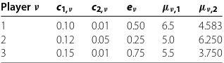
Example . This example is a river basin pollution game also taken from []. There are three players, each player controls a single variablexν∈ . The objective functions are
given by
θν(x) =xνcν+cνxν–d+d
x+x+x
Table 1 Numerical results for Example 4.1
x1 x2 α(x, y)
Table 2 Numerical results for Example 4.2
x1 x2 α(x, y)
[image:13.595.218.377.180.225.2]1e–1 5.333334 5.333333 1.848689e–005 1e–5 5.333333 5.333333 1.851667e–009 1e–8 5.333334 5.333331 1.067513e–012
Table 3 Values of constants for Example 4.3
Playerν c1,ν c2,ν eν μν,1 μν,2
1 0.10 0.01 0.50 6.5 4.583
2 0.12 0.05 0.25 5.0 6.250
3 0.15 0.01 0.75 5.5 3.750
Table 4 Numerical results for Example 4.3
x1 x2 x3 α(x, y)
1e–1 21.148268 16.029412 2.722755 0.050083 1e–5 21.142311 16.026439 2.728349 5.000023e–004 1e–8 21.143711 16.029660 2.726270 3.893246e–008
Table 5 Numerical results for Example 4.4
x1 x2 x3 α(x, y)
1e–1 0.090697 0.090697 0.090697 8.776339e–005 1e–5 0.089987 0.089987 0.089987 2.147441e–006 1e–8 0.090001 0.090001 0.090001 5.020587e–010
forν= , , , and the constraints are
μex+μex+μex≤K, μex+μex+μex≤K.
The economic constantsdandddetermine the inverse demand law and set to . and ., respectively. Values for constantsc,ν,c,ν,eν,μν,, andμν,are given in Table , and
K=K= .
Example . This test problem is an Internet switching model introduced by Kesselman
et al.[]. There areNplayers, the cost function of each player is given by
θν(x) = x
ν
B –
xν !N
ν=xν ,
with constraintsxν≥.,ν= , . . . ,N, and!N
ν=xν≤B. We setN= ,B= . The ex-act solution of this problem is x∗= (., ., . . . , .)T. We only state the first three
components ofxin Table .
Example . Let us consider the following GNEP. There are two players in the game, where player controls a two-dimensional variablex= (x
,x)T∈ and player controls a one-dimensional variablex=x
∈ . The problem is
min x,x
x+xx+x+ (x+x)x– x– x
Table 6 Numerical results for Example 4.5
x1 x2 x3 α(x, y)
1e–1 0.026144 10.972252 7.972330 0.121529 1e–5 0.000640 10.999360 7.999360 1.133698e–005 1e–8 0.000026 10.999974 7.999974 1.252339e–008 1e–10 0.000007 10.999993 7.999993 2.532424e–009
Table 7 Values of constants for Example 4.6
Playerν 1 2 3 4 5 6
ci 0.04 0.035 0.125 0.0166 0.05 0.05
di 2 1.75 1 3.25 3 3
ei 0 0 0 0 0 0
x+ x–x≤,
x+ x+x≤,
min x
x+ (x+x)x– x
s.t.x≥,
x+ x–x≤,
x+ x+x≤.
The problem has infinitely many solutions given by
(α, –α, –α)|α∈[, ],
but it has only one normalized Nash equilibrium atα= .
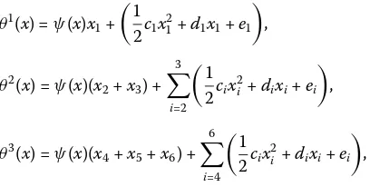
Example . This GNEP from [] is the electricity market problem. This model has three players, player controls a single variablex∈ , player controls a two-dimensional vector x = (x,x), and player controls a three-dimensional decision variable x = (x,x,x). Let
x=x,x,x,x,x,xT= (x,x,x,x,x,x)T.
The utility functions are given by
θ(x) =ψ(x)x+
cx
+dx+e
,
θ(x) =ψ(x)(x+x) +
i=
cix
i +dixi+ei
,
θ(x) =ψ(x)(x+x+x) +
i=
cix
i +dixi+ei
,
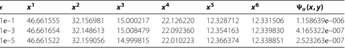
[image:14.595.138.342.610.713.2]Table 8 Numerical results for Example 4.6
x1 x2 x3 x4 x5 x6 α(x, y)
1e–1 46.661555 32.156981 15.000217 22.126220 12.328712 12.331506 1.158639e–006 1e–3 46.661654 32.148613 15.008479 22.092360 12.354163 12.339830 4.165322e–007 1e–5 46.661522 32.159056 14.999815 22.010223 12.366374 12.338851 2.523263e–007
The constraints are
≤x≤, ≤x≤, ≤x≤,
≤x≤, ≤x≤, ≤x≤.
Table is for the corresponding numerical results.
The numerical experiments show that the method proposed in this paper is imple-mentable for solving GNEPs with jointly convex constraints.
5 Remarks
The main idea of this paper is to try use a smoothing method to solve the GNEP. Based on the regularized Nikaido-Isoda function, we reformulate the set of normalized Nash equilibria, which is a subset of the generalized Nash equilibria, as solutions of a MPCC and we solve the MPCC by a smoothing method. There are some problems as regards the smoothing method worth further investigating:
(i) In this paper, some conditions are given to establish the convergence of the smoothing method by showing that any accumulation point of the generated sequence is a M-stationary point of the MPCC. For the next step, less strict assumptions than Theorem . to obtain the results of Theorem . are worth considering.
(ii) Based on the special structure of the MPCC defined in (.), can we derive convergence results tailored to the GNEP, which may possibly be stronger than those known for the MPCC? This problem is worth studying.
Competing interests
The authors declare that they have no competing interests.
Authors’ contributions
JH and J-FL carried out the design of the study and performed the analysis. Z-CW participated in its design and coordination. All authors read and approved the final manuscript.
Author details
1Science College, Inner Mongolia University of Technology, Hohhot, 010051, China.2Management College, Inner Mongolia University of Technology, Hohhot, 010051, China.
Acknowledgements
The research was supported by the Technology Research plan of Inner Mongolia under project Nos. 20130603 and 20120812.
Received: 15 December 2014 Accepted: 23 February 2015 References
1. Debreu, G: A social equilibrium existence theorem. Proc. Natl. Acad. Sci. USA38, 886-893 (1952)
2. Altman, E, Wynter, L: Equilibrium games, and pricing in transportation and telecommunication networks. Netw. Spat. Econ.4, 7-21 (2004)
4. Krawczyk, JB: Coupled constraint Nash equilibria in environmental games. Resour. Energy Econ.27, 157-181 (2005) 5. Facchinei, F, Pang, JS: Finite-Dimensional Variational Inequalities and Complementarity Problems, vol. I. Springer, New
York (2003)
6. Facchinei, F, Pang, JS: Finite-Dimensional Variational Inequalities and Complementarity Problems, vol. II. Springer, New York (2003)
7. Harker, PT: Generalized Nash games and quasi-variational inequalities. Eur. J. Oper. Res.54, 81-94 (1991)
8. Facchinei, F, Pang, JS: Exact penalty functions for generalized Nash problems. In: Large-Scale Nonlinear Optimization. Nonconvex Optimization and Its Applications, vol. 83, pp. 115-126 (2006)
9. Facchinei, F, Kanzow, C: Penalty methods for the solution of generalized Nash equilibrium problems. SIAM J. Optim.
20, 2228-2253 (2010)
10. Krawczyk, JB, Uryasev, S: Relaxation algorithms to find Nash equilibria with economic applications. Environ. Model. Assess.5, 63-73 (2000)
11. Uryasev, S, Rubinstein, RY: On relaxation algorithms in computation of noncooperative equilibria. IEEE Trans. Autom. Control39, 1263-1267 (1994)
12. Zhang, JZ, Qu, B, Xiu, NH: Some projection-like methods for the generalized Nash equilibria. Comput. Optim. Appl.
45, 89-109 (2010)
13. Gürkan, G, Pang, JS: Approximations of Nash equilibria. Math. Program.117, 223-253 (2009)
14. Heusinger, AV, Kanzow, C: Optimization reformulations of the generalized Nash equilibrium problem using Nikaido-Isoda-type functions. Comput. Optim. Appl.43, 353-377 (2009)
15. Fukushima, M, Pang, JS: Convergence of a smoothing continuation method for mathematical programs with complementarity constraints. In: Ill-Posed Variational Problems and Regularization Techniques, pp. 99-110. Springer, Berlin (1999)
16. Facchinei, F, Fischer, A, Piccialli, V: Generalized Nash equilibrium problems and Newton methods. Math. Program.117, 163-194 (2009)
17. Kesselman, A, Leonardi, S, Bonifaci, V: Game-theoretic analysis of Internet switching with selfish users. In: Internet and Network Economics. Lecture Notes in Computer Science, vol. 3828, pp. 236-245. Springer, Berlin (2005)