Artificial Neural Network Based System for PET Volume Segmentation

(1)

Volume 2010, Article ID 105610,11pages doi:10.1155/2010/105610

Research Article

Artificial Neural Network-Based System for

PET Volume Segmentation

Mhd Saeed Sharif,

1

_{Maysam Abbod,}

1

_{Abbes Amira,}

2

_{and Habib Zaidi}

3, 4

1_{Department of Electronic and Computer Engineering, School of Engineering and Design, Brunel University, West London,}

Uxbridge UB8 3PH, UK

2_{Nanotechnology and Integrated Bioengineering Centre, University of Ulster, County Antrim BT37 0QB, UK}

3_{Division of Nuclear Medicine, Geneva University Hospital, 1211 Geneva, Switzerland}

4_{Geneva Neuroscience Center, Geneva University, 1211 Geneva, Switzerland}

Correspondence should be addressed to Mhd Saeed Sharif,[email protected]

Received 14 May 2010; Revised 30 July 2010; Accepted 22 August 2010

Academic Editor: Yue Wang

Copyright © 2010 Mhd Saeed Sharif et al. This is an open access article distributed under the Creative Commons Attribution License, which permits unrestricted use, distribution, and reproduction in any medium, provided the original work is properly cited.

Tumour detection, classification, and quantification in positron emission tomography (PET) imaging at early stage of disease are important issues for clinical diagnosis, assessment of response to treatment, and radiotherapy planning. Many techniques have been proposed for segmenting medical imaging data; however, some of the approaches have poor performance, large inaccuracy, and require substantial computation time for analysing large medical volumes. Artificial intelligence (AI) approaches can provide improved accuracy and save decent amount of time. Artificial neural networks (ANNs), as one of the best AI techniques, have the capability to classify and quantify precisely lesions and model the clinical evaluation for a specific problem. This paper presents a novel application of ANNs in the wavelet domain for PET volume segmentation. ANN performance evaluation using

diﬀerent training algorithms in both spatial and wavelet domains with a diﬀerent number of neurons in the hidden layer is

also presented. The best number of neurons in the hidden layer is determined according to the experimental results, which is also stated Levenberg-Marquardt backpropagation training algorithm as the best training approach for the proposed application. The proposed intelligent system results are compared with those obtained using conventional techniques including thresholding and clustering based approaches. Experimental and Monte Carlo simulated PET phantom data sets and clinical PET volumes of nonsmall cell lung cancer patients were utilised to validate the proposed algorithm which has demonstrated promising results.

1. Introduction

Medical images can be obtained using various modali-ties such as positron emission tomography (PET), single-photon emission computed tomography (SPECT), com-puted tomography (CT), magnetic resonance imaging (MRI), and ultrasound (US). PET is a molecular imaging technique used to probe physiological functions at the molecular level rather than to look at anatomy through the use of trace elements such as carbon, oxygen, and nitrogen which have a high abundance within the human body. PET plays a central role in the management of oncological patients beside the other main components such as diagnosis, staging, treatment, prognosis, and followup. Owing to its high sensitivity and specificity, PET is eﬀective in

targeting specific functional or metabolic signatures that may be associated with various diseases. Among all diagnostic and therapeutic procedures, PET is unique in the sense that it is based on molecular and pathophysiological mechanisms and employs radioactively labeled biological molecules as tracers to study the pathophysiology of the tumour in vivo to direct treatment and assess response to therapy. The leading current area of clinical use of PET is in oncology, where

18_{F-fluorodeoxyglucose (FDG) remains the most widely used}

tracer. FDG-PET has already had a large valuable eﬀect on cancer staging and treatment, and its use in clinical oncology practice continues to evolve [1–5].

(2)

information can be accurately quantified and extracted from the analysed volume. On the other hand, the increasing number of patient scans beside the widespread application of PET have raised the urgent need for eﬀective volume analysis techniques to aid clinicians in clinical diagnosis and set the proper plan for treatment. Analysing and extracting the proper information from PET volumes can be performed by deploying image segmentation and classification approaches which provide richer information than that obtained directly from qualitative assessment alone performed on the original PET volumes [6]. The need for accurate and fast analysis for medical volume segmentation leads to exploit artificial intelligence (AI) techniques. These include artificial neural networks (ANN), expert systems, robotics, genetic algo-rithms, intelligent agents, logic programming, fuzzy logic, neurofuzzy, natural language processing, and automatic speech recognition [7,8].

ANN is one of the powerful AI techniques that has the capability to learn from a set of data and construct weight matrices to represent the learning patterns. ANN has great success in many applications including pattern classification, decision making, forecasting, and adaptive control. Many research studies have been carried out in the medical field utilising ANN for medical image segmentation and classifi-cation with diﬀerent medical imaging modalities. Multilayer perceptron (MLP) neural network (NN) have been used by [9] to identify breast nodule malignancy using sonographic images. A multiple classifier system using five NNs and five sets of texture features extraction for the characterization of hepatic tissue from CT images is presented in [10]. Kohonen self-organizing NN for segmentation and a multi-layer backpropagation NN for classification for multispectral MRI images have been used in [11]. Kohonen NN was also used for image segmentation in [12]. Computer-aided diagnostic (CAD) scheme to detect lung nodules using a multiresolution massive training artificial neural network (MTANN) is presented in [13].

The aim of this paper is to develop a robust, efficient PET volume segmentation system using ANN. The proposed system is evaluated using different training algorithms and its performance assessed using different metrics. ANN outputs are also compared with the outputs of conventional approaches including thresholding and clustering using experimental PET phantom studies and clinical volumes of nonsmall cell lung cancer patients.

This paper is organised as follows. Section 2 presents mathematical background for the selected approaches. The materials and methods used are described in Section 3. Experimental results and their discussion are given in section 4, and finally some conclusions are presented inSection 5.

2. Mathematical Background

2.1. Mathematical Model of a Neuron. ANN is a

mathemat-ical model which emulates the activity of biologmathemat-ical neural networks in the human brain. It consists of two or several layers each one has many interconnected group of neurons. Each neuron in the ANN has a number of inputs (the input

vectorP) and one output (Y). The input vector elements are multiplied by weightsw1,1,w1,2,. . .,w1,R, and the weighted

values are fed to the summing junction. Their sum is simply the dot product (W.P) of the single-row matrixW and the vectorP. The neuron has a biasb, which is summed with the weighted inputs to form the net inputn. This sum,n, is the argument of the transfer function f [14]

n=

R

i=1

w1,i·pi+b, (1)

Y =f(W·P+b), (2)

Yj= f

⎡

⎣R

i=1

w1,i

j.pij+b

⎤

⎦_. ₍₃₎

The learning process can be summarized in the following steps: (1) the initial weights are randomly assigned, (2) the neuron is activated by applying inputs vector and desired output (Yd), and (3) calculation of the actual output (Y) at iteration j=1 as illustrated in (3), where iteration jrefers to the jth training example presented to the neuron. The following step is to update the weights to obtain the output consistent with the training examples, as illustrated in

w1,i

j+ 1=w1,i

j+Δw1,i

j, (4)

where Δw1,i(j) is the weight correction at iteration j. The

weight correction is computed by using the delta rule in

Δw1,i

j=α∗pij∗ej, (5)

whereαis the learning rate ande(j) is the error which can be given by

ej=Ydj−Yj. (6)

Finally, the iteration jis increased by one, and the previous two steps are repeated until the convergence is reached.

2.2. Thresholding

2.2.1. Hard Thresholding. Thresholding is the simplest

pre-cursory technique for image segmentation. This method-ology attempts to determine an intensity value that can separate the slice g(x,y) into two parts [15]. All voxels with intensities f(x,y) larger than the threshold valueTare allocated into one class, and all the others into another class.

gx,y= ⎧ ⎨ ⎩

fx,y if fx,y> T,

0 if fx,y< T. (7)

(3)

2.2.2. Soft Thresholding. Soft thresholding is more complex

process compared to hard thresholding. This approach replaces each voxel which has a greater value than the threshold value by the diﬀerence between the threshold and the current voxel values. Soft thresholding could put into evidence some important regions as the region of interest (ROI) in this study.

2.2.3. Adaptive Thresholding. Otsu’s method has been used

as a third approach, which chooses the threshold that minimizes the intraclass variance of the black and white voxels in the volume [18]. Likewise, other variants of adaptive thresholding based on source-to-background ratio were also reported [4].

2.3. Multiresolution Analysis. Multiresolution analysis

(MRA) is designed to give good time resolution and poor frequency resolution at high frequencies, and poor time resolution and good frequency resolution at low frequencies. It enables the exploitation of slice characteristics associated with a particular resolution level, which may not be detected using other analysis techniques [19–21]. The wavelet transform for a function f(t) can be defined as follows:

Xψ(a,b)=

_∞

−∞ f(t)ψ(a,b)(t)dt, (8)

where

ψ(a,b)(t)=

1

√

aψ

t−b

a

. (9)

The parameters a, b are called the scaling and shifting parameters, respectively [20,22]. Haar wavelet filter will be used in the experimental study at different levels of decom-position. The Haar wavelet transform (HWT) of a two-dimensional slice can be performed using two approaches: the first one is called standard decomposition of a slice, where the one-dimensional HWT is applied to each row of voxel values followed by another one-dimensional HWT on the column of the processed slice. The other approach is called nonstandard decomposition, which alternates between the one-dimensional HWT operations on rows and columns. HWT serves as a prototype for all other wavelet transforms. Like all wavelet transforms, HWT decomposes a slice into four subimages of half the original size. HWT is conceptually simple, fast, memory efficient, and can be reversed without the edge effects that are associated with other wavelet transforms. HWT is a matrix-vector-based operation and can be formulated as follows:

H=1

2

⎛

⎝1 1

1 −1

⎞

⎠_, ₍₁₀₎

O=I×H, (11)

O=(IH)THT =HT_IH_, ₍₁₂₎

I=H−1T_OH−1_, ₍₁₃₎

where I is 2 × 2 input matrix, H contains the Haar coeﬃcients, and O is the output matrix. Equations (12) and (13) show the transposed and reconstructed matrices, respectively. MRA has been used in the literature for diﬀerent applications [22–24].

2.4. Clustering. Clustering techniques aim to classify each

voxel in a volume into the proper cluster, then these clusters are mapped to display the segmented volume. The most commonly used clustering technique is the K -means method, which clusters n voxels into K clusters (K less than n) [25]. This algorithm chooses the number of clusters, K, then randomly generates K clusters and determines the cluster centers. The next step is assigning each point in the volume to the nearest cluster center, and finally recompute the new cluster centers. The two previous steps are repeated until the minimum variance criterion is achieved. This approach is similar to the expectation-maximization algorithm for Gaussian mixture in which they both attempt to find the centers of clusters in the volume. Its main objective is to achieve a minimum intracluster variance

V

V=

K

i=1

xj∈Si

xj−μi2, (14)

whereK is the number of clusters,S = 1, 2,. . .,K, and μi

is the mean of all voxels in the clusteri.K-means approach has been used with other techniques for clustering medical images [26].

3. Materials and Methods

3.1. The Proposed System. The proposed medical volume

(4)

3D PET volumes

Preprocessing stage

Thresholding

Clustering

MRA

Hard

Soft

Adaptive

Choose the Number of clusters

ANN

Segmented volumes

Figure 1: Proposed system for PET volume segmentation.

1

0

−1

n

(a)

1

0

−1

n

(b)

Figure 2: Activation functions: (a) Tangent-sigmoid function, (b) Linear function.

0 0.01 0.02 0.03 0.04 0.05 0.06 0.07 0.08 0.09 0.1

Pe

rf

o

rm

an

ce

(M

S

E

)

0 10 20 30 40 50 60 70 80 90 100 110 Number of neurons

Figure 3: Evaluation of the number of neurons in the first hidden layer with neural network performance using MSE.

3.2. Phantom Studies. In this study, PET volumes containing

simulated tumour have been utilised. Two phantom data sets have been used. The first data set is obtained using NEMA IEC image quality body phantom which consists of an ellip-tical water-filled cavity with six spherical inserts suspended by plastic rods of volumes 0.5, 1.2, 2.6, 5.6, 11.5, and 26.5 ml (inner diameters of 10, 13, 17, 22, 28, and 37 mm). The voxel size is 4.07 mm × 4.07 mm × 5 mm, while the size

0 2 4 6 8 10 12 14 16 18 20 22 24 26 28 30

Vo

lu

m

e

(m

L

)

0 2 4 6 8

Spheres number True volume

Adaptive

Soft Hard

Figure 4: The segmented volume for all spheres in data set 1 using adaptive, soft, and hard thresholding approaches, respectively.

(5)

(a) (b)

[image:5.600.153.448.73.343.2]

(c) (d)

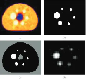
Figure 5: Phantom data set 1: (a) Original PET image (168×168), (b) thresholded image (168×168), (C) clustered image (168×168),

[image:5.600.51.291.412.478.2]

(d) segmented image (84×84) using ANN and MRA, zoomed by a factor of 2.

Table 1: Tumours characteristics for the second data set.

Tumour Isotropic Nonisotropic

Number Position Size Position Size

1 slice 68 2 voxels slice 142 2 voxels

CT-based attenuation correction was used to reconstruct the PET emission data. The default parameters used were ordered OSEM iterative reconstruction with four iterations and eight subsets followed by a postprocessing Gaussian filter (kernel full-width half-maximal height, 5 mm).

The second data set consists of Monte Carlo simulations of the Zubal antropommorphic model where two volumes were generated [33]. The first volume contains a matrix with isotropic voxels, the size of this volume is 128×128×180. The second volume contains the same matrix of the first one but with nonisotropic voxels having a matrix size of 128×

128 × 375. The voxel size in both volumes is 5.0625 mm

× 5.0625 mm× 2.4250 mm. The second data volume has 3 tumours in the lungs whose characteristics are given in

Table 1.

3.3. Clinical PET Studies. Clinical PET volumes of patients

with histologically proven NSCLC (clinical Stage Ib-IIIb) who have undertaken a diagnostic whole-body PET/CT scan were used for assessment of the proposed segmentation technique [34]. Patients fasted no less than 6 hours before

PET/CT scanning. The standard protocol involved intra-venous injection of18_{F-FDG followed by a physiologic saline}

(10 ml). The injected FDG activity was adjusted according to patient’s weight using the following formula: A (Mbq)

= weight (Kg) 4 + 20. After 45 min uptake time, free-breathing PET and CT images were acquired. The data were reconstructed using the same procedure described for the phantom studies. The maximal tumour diameters measured from the macroscopic examination of the surgical specimen served as ground truth for comparison with the maximum diameter estimated by the proposed segmentation technique. The voxel size is 5.31 mm×5.31 mm×5 mm, while the size of the obtained clinical volume is 128×128×178.

4. Results and Discussion

4.1. NEMA Image Quality Phantom. An experimental study

(6)

0 0.2 0.4 0.6 0.8 1

15 10

5

0 0 5

10 15 (a)

0 0.2 0.4 0.6 0.8 1

15 10

5

0 0 5

10 15 (b)

0 0.2 0.4 0.6 0.8 1

15 10

5

0 0 5

10 15 (c)

0 0.2 0.4 0.6 0.8 1

15 10

5

0 0 5

10 15 (d)

0 0.1 0.2 0.3 0.4 0.5 0.6

15 10

5

0 0 5

10 15 (e)

0 0.1 0.15 0.2 0.250.3 0.35

15 10

5

0 0 5

10 15 (f)

Figure 6: Segmented sphere surface plot for phantom data set 1. Voxel values scaled in [0..1] on Z axis, and voxels number is within [0..12] on X and Y axes: (a) sphere 1, (b) sphere 2, (c) sphere 3, (d) sphere 4, (e) sphere 5, and (f) sphere 6.

Tumour

(a) (b)

(c) (d)

Figure 7: Phantom data set 2. (Tumour 1): (a) Original PET image (128×128), (b) thresholded image (128×128), (C) clustered image

(128×128), (d) segmented image (64×64) using ANN and MRA, zoomed by a factor of 2, where tumour 1 (2 voxel) is detected.

except the output layer where the linear activation function is used. The two activation functions are illustrated inFigure 2. Levenberg-Marquardt backpropagation training algorithm has been used during the evaluation of neurons numbers in the hidden layer [35] to validate the best design for the ANN, which is suitable for the proposed application.Figure 3

presents the number of neurons in the first hidden layer with the performance measured using mean-squared error (MSE) at 1000 iterations. The results obtained after this evaluation shows that the best number of the hidden neurons which

corresponds to the smallest MSE, and good ANN outputs is 70 hidden neurons.

(7)

1 2 Output cl ass 1 2 Target class 64 44.4% 0 0% 100% 0% 1 0.7% 79 54.9%

98.8% 1.2%

98.5% 1.5%

100% 0%

99.3% 0.7%

(a) 1 2 Output cl ass 1 2 Target class 2 0% 0 0% 100% 0% 0 0% 4094 100% 100% 0% 100% 0% 100% 0% 100% 0% (b) 1 2 Output cl ass 1 2 Target class 3 0.1% 0 0% 100% 0% 0 0% 4093 100% 100% 0% 100% 0% 100% 0% 100% 0% (c) 1 2 Output cl ass 1 2 Target class 2 0.1% 0 0% 100% 0% 0 0% 4094 100% 100% 0% 100% 0% 100% 0% 100% 0% (d)

Figure 8: Confusion matrix: (a) for phantom data set 1, sphere 1, (b) phantom data set 2, tumour 1, (c) phantom data set 2, tumour 2, and (d) for phantom data set 2, tumour 3.

restarts (CGB) [38], conjugate gradient backpropagation with Fletcher-Reeves updates (CGF) [39], conjugate gradient backpropagation with Polak-Ribire updates (CGP) [39], gra-dient descent backpropagation (GD) [40], gradient descent with momentum backpropagation (GDM) [41], gradient descent with adaptive learning rate backpropagation (GDA) [42], gradient descent with momentum and adaptive learn-ing rate backpropagation (GDX) [43], Levenberg-Marquardt backpropagation (LM) [35], one-step secant backpropaga-tion (OSS) [44], random order incremental training with learning functions (R), resilient backpropagation (RP) [45], and scaled conjugate gradient backpropagation (SCG) [46]. The average of the performance and the required time for each of these training algorithms are presented inTable 2, this experiment has been repeated for 10 times and the standard deviation for the performance achieved is 4.15E-07. The best outputs associated with the best performance was achieved using Levenberg-Marquardt backpropagation training algorithm. This algorithm is using a combination of techniques which allows the NN to be trained eﬃciently. This combination includes backpropagation, gradient descent approach, and Gauss-Newton technique [47,48].

(8)

(a) (b)

(c) (d)

Figure 9: Illustration of algorithm performance on clinical PET data showing: (a) original PET image (128×128), (b) thresholded image

(128×128), (C) clustered image (128×128), and (d) segmented image (64×64) using ANN and MRA, zoomed by a factor of 2.

Table 2: Evaluation of the eﬀect of diﬀerent training algorithms

on the performance of multilayer feedforward NN with 144-70-1 topology.

Training function Time (sec) Performance (MSE)

BFG 58 0.000426

BR 35 3.69e-6

CGB 11 0.0128

CGF 11 0.0156

CGP 13 0.0160

GD 6 0.117

GDM 6 0.100

GDA 6 0.0950

GDX 6 0.0383

LM 27 1.32E-7

OSS 13 0.0198

R 226 0.0503

RP 6 0.0183

SCG 10 0.0154

of the original size. The ANN achieved good performance with very small MSE, 2.39E-16.

An objective evaluation of the artificial intelligence system (AIS) outputs has been performed by comparing the sphere computed volume (CV) with its true original volume (TV). The experimental results have been repeated 10 times, and the average of the sphere volume measured using ANN is calculated. The standard deviation for the volume of sphere 1 is 0.0971, for sphere 2 is 0.1170, for sphere 3 is 0.1185, for sphere 4 is 0.1232, for sphere 5

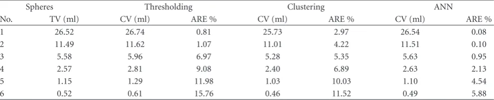
is 0.1258, and for sphere 6 is 0.1293. The CV obtained from the ANN, and the percentage of the absolute relative error (ARE %) for each sphere are presented in Table 3. ANN has clearly detected all spheres, where spheres 1, 2, and 3 are accurately segmented whereas spheres 4 is overestimated, and sphere 5 and 6 are underestimated. It is worth mentioning that the proposed system has shown better performance compared to the thresholding and clustering based approaches which are used as ground truth. Adaptive, soft, and hard thresholding approaches have been also used to perform the segmentation. The best results obtained from these approaches is by using adaptive threshold method which is used for the comparison with the other assessed techniques.Figure 4presents the obtained spheres volumes using three thresholding approaches. Table 3 illustrates a comparison between the assessed approaches in term of ARE percentage. Thresholding approach has overestimated the volume of all spheres, while the exploitation of K-means clustering approach underestimates the volume of all spheres, particularly spheres 5 and 6.

The segmented slices from thresholding, clustering and ANN in the wavelet domain are illustrated in Figure 5, where Figure 5(d)is zoomed for illustration purpose. The three-dimensional shaded surface for each segmented sphere obtained from ANN are plotted inFigure 6, where the voxel values are scaled in [0..1] on Z axis and voxels number is within [0..12] on the remaining two axes.

4.2. Simulated Zubal Phantom. The proposed segmentation

(9)

[image:9.600.53.549.100.201.2]

Table 3: Comparison of sphere volumes and ARE between TV and CV for diﬀerent segmentation algorithms assessed including thresholding, clustering and ANN.

Spheres Thresholding Clustering ANN

No. TV (ml) CV (ml) ARE % CV (ml) ARE % CV (ml) ARE %

1 26.52 26.74 0.81 25.73 2.97 26.54 0.08

2 11.49 11.62 1.07 11.01 4.22 11.51 0.10

3 5.58 5.96 6.97 5.28 5.35 5.63 0.95

4 2.57 2.81 9.08 2.40 6.89 2.63 2.13

5 1.15 1.29 11.98 1.03 10.03 1.10 4.54

6 0.52 0.61 15.76 0.46 11.52 0.49 5.88

of 2 voxels was clearly detected in slice 68. Figure 7shows the segmented slices from thresholding, clustering, and ANN in the wavelet domain for this tumour. The second and third tumours with size 3 and 2 voxels, respectively, were also clearly detected in slice 57 and 74, respectively. Similar results have been achieved for detecting tumours in the second data set with nonisotropic voxels. On the other hand similar segmented slices have been obtained using ANN in the spatial domain, however, more computational time is required for processing all data sets in this domain.

4.3. Performance Evaluation. In the field of AI a number

of performance metrics can be employed to evaluate the performance of ANN. A confusion matrix is a visualisation tool typically used in supervised and unsupervised learning approaches. Each row of the matrix represents the instances in a predicted class, while each column represents the instances in an actual class. One benefit of a confusion matrix is that it is easy to see if the system is confusing two classes (the tumour and the remaining tissues). The confusion matrix for the first data set shows that 1 voxel out of 65 ones in the first segmented sphere was misclassified,

Figure 8(a). Where the percent in the green box refers to each

class prediction accuracy. While the percent in the pink box refers to the misclassified voxels accuracy in each class. The gray boxes represent the percents of classified voxels numbers in each class in green, and the percent of the error in each class in red. The blue box represents the total percent of all classes in green and the total error in these classes in red. All the numbers in the confusion matrix are represented as a percentage.

The confusion matrix for the second data set, tumour 1 is illustrated inFigure 8(b). The two voxels of this tumour were precisely classified in one class and the remaining voxels (4094) classified in the other class. The confusion matrix for the second data set, tumour 2, shows that the 3 voxels were precisely classified as a first class and the remaining voxels (4093) classified in the other class. The obtained result is presented inFigure 8(c), whileFigure 8(d)illustrates the confusion matrix for the second data set, tumour 3. The two voxels of tumour 3 were precisely classified as a first class and the remaining voxels (4094) classified in the other class.

The other performance checking approach is receiver operating characteristic (ROC). This approach can be repre-sented by plotting the fraction of true positives rate (TPR)

versus the fraction of false positives rate (FPR), where the perfect point in the ROC curve is the point (0,1). The ROC curve for the first data set is located near the perfect point and the FPR for the sphere voxels number is near the 0 point. Perfect ROC has been obtained for the second data set and the FPR for tumour voxels number is 0.

4.4. Clinical PET Studies. The proposed approaches have

been also tested on clinical PET volumes of nonsmall cell lung cancer patients. A subjective evaluation based on the clinical knowledge has been carried out for the output of the proposed approaches. The tumour in these slices has a maximum diameter on the y-axis of 90 mm (estimated by histology). The segmented tumour using ANN in spatial domain and wavelet domain (after scaling) has a diameter of 90.1 mm. The segmented volumes using the proposed approaches outlines a well defined contour as illustrated in

Figure 9.

5. Conclusions

An artificial intelligence system based on multilayer artificial neural networks was proposed for PET volume segmen-tation. Diﬀerent training algorithms have been utilised in this study to validate the best algorithm for the targeted application. Two PET phantom data sets and a clinical PET volume of nonsmall cell lung cancer patient have been used to evaluate the performance of the proposed system. Objective and subjective evaluation for the system outputs have been carried out. Confusion matrix and receiver operating characteristic were also used to judge the performance of the trained neural network. Experimental and simulated phantom results have shown a good perfor-mance for the ANN in detecting the tumours in spatial and wavelet domains for both phantom and clinical PET volumes. Accurate tumour quantification was also achieved through this system. Ongoing research is focusing on further validation of the proposed algorithm in a clinical setting and the exploitation of other artificial intelligence tools and feature extraction techniques.

Acknowledgment

(10)

References

[1] D. Mankoﬀ, M. Muzi, and H. Zaidi, “Quantitative

analy-sis in nuclear oncologic imaging,” in Quantitative Analyanaly-sis in Nuclear Medicine Imaging, H. Zaidi, Ed., pp. 494–536, Springer, New York, NY, USA, 2006.

[2] D. W. G. Montgomery, A. Amira, and H. Zaidi, “Fully automated segmentation of oncological PET volumes using a combined multiscale and statistical model,” Medical Physics, vol. 34, no. 2, pp. 722–736, 2007.

[3] M. Aristophanous, B. C. Penney, and C. A. Pelizzari, “The development and testing of a digital PET phantom for the evaluation of tumor volume segmentation techniques,” Medical Physics, vol. 35, no. 7, pp. 3331–3342, 2008.

[4] H. Vees, S. Senthamizhchelvan, R. Miralbell, D. C. Weber, O. Ratib, and H. Zaidi, “Assessment of various strategies for 18F-FET PET-guided delineation of target volumes in high-grade glioma patients,” European Journal of Nuclear Medicine and Molecular Imaging, vol. 36, no. 2, pp. 182–193, 2009.

[5] S. Basu, “Selecting the optimal image segmentation strategy in the era of multitracer multimodality imaging: a critical step for image-guided radiation therapy,” European Journal of Nuclear Medicine and Molecular Imaging, vol. 36, no. 2, pp. 180–181, 2009.

[6] H. Zaidi and I. El Naqa, “PET-guided delineation of radiation therapy treatment volumes: a survey of image segmentation techniques,” European Journal of Nuclear Medicine and Molec-ular Imaging, vol. 37, pp. 1–37, 2010.

[7] G. Dreyfus, Neural Networks Methodology and Applications, Springer, Berlin, Germany, 2005.

[8] M. A. Arbib, The Handbook of Brain Theory and Neural Networks, Massachusetts Institute of Technology, Cambridge, Mass, USA, 2003.

[9] S. Joo, W. K. Moon, and H. C. Kim, “Computer-aidied diagnosis of solid breast nodules on ultrasound with digital image processing and artificial neural network,” in Proceedings of the 26th Annual International Conference of the IEEE Engineering in Medicine and Biology Society (EMBS ’04), pp. 1397–1400, 2004.

[10] S. G. Mougiakakou, I. Valavanis, K. S. Nikita, A. Nikita, and D. Kelekis, “Characterization of CT liver lesions based on texture features and a multiple neural network classification scheme,” in Proceedings of the 25th Annual International Conference of the IEEE Engineering in Medicine and Biology Society (EMBS ’03), vol. 2, pp. 1287–1290, 2003.

[11] W. E. Reddick, J. O. Glass, E. N. Cook, T. D. Elkin, and R. J. Deaton, “Automated segmentation and classification of multispectral magnetic resonance images of brain using artificial neural networks,” IEEE Transactions on Medical Imaging, vol. 16, no. 6, pp. 911–918, 1997.

[12] C. C. Reyes-Aldasoro and A. Aldeco, “Image segmentation and compression using neural networks,” in Advances in Artificial Perception and Robotics CIMAT, 2000.

[13] K. Suzuki, H. Abe, H. MacMahon, and K. Doi, “Image-processing technique for suppressing ribs in chest radio-graphs by means of massive training artificial neural network (MTANN),” IEEE Transactions on Medical Imaging, vol. 25, no. 4, pp. 406–416, 2006.

[14] G. F. Luger, Artificial Intelligence: Structures and Strategies for Complex Problem Solving, Pearson Education Inc., 2009. [15] P. K. Sahoo, S. Soltani, and A. K. C. Wong, “A survey

of thresholding techniques,” Computer Vision, Graphics and Image Processing, vol. 41, no. 2, pp. 233–260, 1988.

[16] A. Kanakatte, J. Gubbi, N. Mani, T. Kron, and D. Binns, “A pilot study of automatic lung tumor segmentation from positron emission tomography images using standard uptake values,” in Proceedings of the IEEE Symposium on Computa-tional Intelligence in Image and Signal Processing (CIISP ’07), pp. 363–368, 2007.

[17] M. Sezgin and B. Sankur, “Survey over image thresholding techniques and quantitative performance evaluation,” Journal of Electronic Imaging, vol. 13, no. 1, pp. 146–168, 2004. [18] N. Otsu, “A threshold selection method from gray-level

his-tograms,” IEEE Transactions on Systems, Man, and Cybernetics, vol. 9, no. 1, pp. 62–66, 1979.

[19] S. G. Mallat, “A theory for multiresolution signal decomposi-tion: the wavelet representation,” IEEE Transactions on Pattern Analysis and Machine Intelligence, vol. 11, no. 7, pp. 674–693, 1989.

[20] R. Gonzalez and R. Woods, Digital Image Processing, Prentice-Hall, Upper Saddle River, NJ, USA, 2001.

[21] A. Amira, S. Chandrasekaran, D. W. G. Montgomery, and I. Servan Uzun, “A segmentation concept for positron emission tomography imaging using multiresolution analysis,”

Neuro-computing, vol. 71, no. 10−12, pp. 1954–1965, 2008.

[22] K. M. Rajpoot and N. M. Rajpoot, “Hyperspectral colon tissue cell classification,” in Medical Imaging, Proceedings of SPIE, 2004.

[23] G. Fan and X.-G. Xia, “Wavelet-based texture analysis and synthesis using hidden Markov models,” IEEE Transactions on Circuits and Systems I, vol. 50, no. 1, pp. 106–120, 2003. [24] H. Liu, Z. Chen, X. Chen, and Y. Chen, “Multiresolution

medical image segmentation based on wavelet transform,” in Proceedings of the 27th Annual International Conference of the IEEE Engineering in Medicine and Biology Society (EMBS ’05), pp. 3418–3421, September 2005.

[25] A. K. Jain and R. C. Dubes, Algorithms for Clustering Data, Prentice-Hall, Upper Saddle River, NJ, USA, 1988.

[26] H. P. Ng, S. H. Ong, K. W. C. Foong, P. S. Goh, and W. L. Nowinski, “Medical image segmentation using k-means clustering and improved watershed algorithm,” in Proceedings of the 7th IEEE Southwest Symposium on Image Analysis and Interpretation, pp. 61–65, March 2006.

[27] C. Jonsson, R. Odh, P.-O. Schnell, and S. A. Larsson, “A comparison of the imaging properties of a 3- and 4-ring bio-graph PET scanner using a novel extended NEMA phantom,” in Proceedings of the IEEE Nuclear Science Symposium and Medical Imaging Conference (NSS-MIC ’07), vol. 4, pp. 2865– 2867, November 2007.

[28] M. D. R. Thomas, D. L. Bailey, and L. Livieratos, “A dual modality approach to quantitative quality control in emission tomography,” Physics in Medicine and Biology, vol. 50, no. 15, pp. N187–N194, 2005.

[29] H. Bergmann, G. Dobrozemsky, G. Minear, R. Nicoletti, and M. Samal, “An inter-laboratory comparison study of image quality of PET scanners using the NEMA NU 2-2001 procedure for assessment of image quality,” Physics in Medicine and Biology, vol. 50, no. 10, pp. 2193–2207, 2005.

[30] H. Herzog, L. Tellmann, C. Hocke, U. Pietrzyk, M. E. Casey, and T. Kawert, “NEMA NU2-2001 guided performance evalu-ation of four siemens ECAT PET scanners,” IEEE Transactions on Nuclear Science, vol. 51, no. 5, pp. 2662–2669, 2004. [31] J. M. Wilson and T. G. Turkington, “Multisphere phantom and

analysis algorithm for PET image quality assessment,” Physics in Medicine and Biology, vol. 53, no. 12, pp. 3267–3278, 2008. [32] H. Zaidi, F. Schoenahl, and O. Ratib, “Geneva PET/CT facility:

(11)

commercial (Biograph 16/64) scanners,” European Journal of Nuclear Medicine and Molecular Imaging, vol. 34, supplement 2, p. S166, 2007.

[33] S. Tome¨ı, A. Reilhac, D. Visvikis et al., “OncoPET-DB: a freely distributed database of realistic simulated whole body 18F-FDG PET images for oncology,” IEEE Transactions on Nuclear Science, vol. 57, no. 1, pp. 246–255, 2010.

[34] A. van Baardwijk, G. Bosmans, L. Boersma et al., “PET-CT-based auto-contouring in non-small-cell lung cancer correlates with pathology and reduces interobserver variability in the delineation of the primary tumor and involved nodal volumes,” International Journal of Radiation Oncology, Biology, Physics, vol. 68, no. 3, pp. 771–778, 2007.

[35] B. G. Kermani, S. S. Schiﬀman, and H. T. Nagle, “Performance

of the Levenberg-Marquardt neural network training method in electronic nose applications,” Sensors and Actuators B, vol. 110, no. 1, pp. 13–22, 2005.

[36] P. E. Gill, W. Murray, and M. H. Wright, Practical Optimiza-tion, Academic Press, New York, NY, USA, 1981.

[37] D. MacKay, “Bayesian interpolation,” Neural Computation, vol. 4, no. 3, pp. 415–447, 1992.

[38] M. J. D. Powell, “Restart procedures for the conjugate gradient method,” Mathematical Programming, vol. 12, no. 1, pp. 241– 254, 1977.

[39] L. E. Scales, Introduction to Non-Linear Optimization, Springer, Berlin, Germany, 1985.

[40] Y. Bengio, P. Simard, and P. Frasconi, “Learning

long-term dependencies with gradient descent is diﬃcult,” IEEE

Transactions on Neural Networks, vol. 5, no. 2, pp. 157–166, 1994.

[41] A. Bhaya and E. Kaszkurewicz, “Steepest descent with momen-tum for quadratic functions is a version of the conjugate gradient method,” Neural Networks, vol. 17, no. 1, pp. 65–71, 2004.

[42] S. Iranmanesh, “A diﬀerential adaptive learning rate method

for back-propagation neural networks,” in Proceedings of the 10th WSEAS International Conference on Neural Networks, 2009.

[43] G. D. Magoulas, M. N. Vrahatis, and G. S. Androulakis, “Improving the convergence of the backpropagation algo-rithm using learning rate adaptation methods,” Neural Com-putation, vol. 11, no. 7, pp. 1769–1796, 1999.

[44] R. Battiti, “First and second order methods for learning: between steepest descent and Newton’s method,” Neural Computation, vol. 4, no. 2, pp. 141–166, 1992.

[45] M. Riedmiller and H. Braun, “A direct adaptive method for faster backpropagation learning: the RPROP algorithm,” in Proceedings of the IEEE International Conference on Neural Networks (ICNN ’93), pp. 586–591, April 1993.

[46] M. F. Moller, “A scaled conjugate gradient algorithm for fast supervised learning,” Neural Networks, vol. 6, no. 4, pp. 525– 533, 1993.

[47] X. Yu, M. O. Efe, and O. Kaynak, “A backpropagation learning framework for feedforward neural networks,” in Proceedings of the IEEE International Symposium on Circuits and Systems (ISCAS ’01), vol. 3, pp. 700–702, May 2001.

(12)

,QWHUQDWLRQDO-RXUQDORI

$HURVSDFH

(QJLQHHULQJ

+LQGDZL3XEOLVKLQJ&RUSRUDWLRQ

KWWSZZZKLQGDZLFRP 9ROXPH

Robotics

Journal of

Hindawi Publishing Corporation

http://www.hindawi.com Volume 201

Active and Passive Electronic Components

Control Science and Engineering

Journal of

Hindawi Publishing Corporation

http://www.hindawi.com Volume 2014 Machinery

Hindawi Publishing Corporation http://www.hindawi.com

Journal of

(QJLQHHULQJ

Volume 201

Submit your manuscripts at

http://www.hindawi.com

VLSI Design

Hindawi Publishing Corporation

http://www.hindawi.com Volume 201

-Hindawi Publishing Corporation

Shock and Vibration

Civil Engineering

Advances in

Acoustics and Vibration Advances in

Electrical and Computer Engineering

Journal of

Advances in OptoElectronics

)JOEBXJ1VCMJTIJOH$PSQPSBUJPO

IUUQXXXIJOEBXJDPN 7PMVNF

The Scientiﬁc

World Journal

Sensors

Journal of

Modelling & Simulation in Engineering

)JOEBXJ1VCMJTIJOH$PSQPSBUJPO

IUUQXXXIJOEBXJDPN 7PMVNF

Chemical Engineering

International Journalof Antennas and Propagation

International Journal of

http://www.hindawi.com Volume 2014 Navigation and Observation

International Journal of

Artificial Neural Network Based System for PET Volume Segmentation

Research Article