Causal Method and Time Series Forecasting model based on Artificial Neural Network

Causal Method and Time Series Forecasting model

based on Artificial Neural Network

Benkachcha.S,

Laboratory LISER, ENSEM, Km 7 BP 8118 Route El Jadida

Casablanca, Morocco

Benhra.j,

Laboratory LISER, ENSEM, Km 7 BP 8118 Route El Jadida

Casablanca, Morocco

El Hassani.H,

École Hassania des Travaux Publics Km 7 Route El Jadida

BP 8108 Casablanca, Maroc

ABSTRACT

This article discusses two methods of dealing with demand variability. First a causal method based on multiple regression and artificial neural networks have been used. The ANN is trained for different structures and the best is retained. Secondly a multilayer perceptron model for time series forecasting is proposed. Several learning rules used to adjust the ANN weights have been evaluated. The results show that the performances obtained by the two methods are very similar. The cost criterion is then used to choose the appropriate model.

General Terms

Feedforward Neural Networks; Multilayer Perceptron; Levenberg-Marquardt backpropagation algorithm. Time series forecasting model and causal method.

Keywords

Demand Forecasting, Supply Chain, Time Series, Causal Method, Multiple Regression, Artificial Neural Networks (ANN).

1.

INTRODUCTION

In any production environment, demand forecasting plays an important role for managing integrated logistics system. It provides valuable information for several logistics activities including purchasing, inventory management, and transportation. In practice there are extensive forecasting techniques available for anticipating the future. This article presents a contribution to improve the quality of forecasts by using Artificial Neural Networks (ANN). It discusses two methods of dealing with demand variability. First a causal method based on multiple regression and artificial neural networks have been used. The ANN is trained for different structures and the best is retained. Secondly a multilayer perceptron model for univariate time series forecasting is proposed. Several learning rules used to adjust the ANN weights have been evaluated. The results show that the performances obtained by the two methods are very similar. The cost criterion is then used to choose the appropriate model.

The rest of the paper is organized as follows. Section 2 reviews the literature in forecasting and the use of Artificial Neural network in this area. Section 3 presents two prediction models: causal method and time series model based on neural networks. Section 4 discusses the results obtained using this methodology in a case study. Section 5 gives the conclusion of the paper.

2.

LITERATURE REVIEW

Quantitative forecasting models can be grouped into two categories: the time series models and causal methods. Time series analysis tries to determine a model that explains the historical demand data and allows extrapolation into the future to provide a forecast in the belief that the demand data represent experience that is repeated over time.

This category includes naïve method, moving average, trend curve analysis, exponential smoothing, and the autoregressive integrated moving averages (ARIMA) models. These techniques are appropriate when we can describe the general patterns or tendencies, without regard to the factors affecting the variable to be forecast (Kesten C. Green & J. Scott Armstrong 2012). One of the reasons for its popularity is the lower cost. Easy to develop and implement, times series models are preferred for they have been used in many applications such as: Economic Forecasting, Sales Forecasting, Budgetary Analysis, Stock Market Analysis, Process and Quality Control and Inventory Studies (GOSASANG V. & all, 2011).On the other hand, the causal methods search for reasons for demand, and are preferred when a set of variables affecting the situation are available (Armstrong, J. S. 2012). Among the models of this category, multiple linear regression uses a predictive causal model that identifies the causal relationships between the predictive (forecast) variable and a set of predictors (causal factors). For example, the customer demand can be predicted through a set of causal factors such as predictors product price, advertising costs, sales promotion, seasonality, etc. (Chase, 1997). Both kinds of models (time series models and the linear causal methods) are easy to develop and implement. However they may not be able to capture the nonlinear pattern in data. Neural Network modelling is a promising alternative to overcome these limitations (Chen, K.Y., 2011). Mitrea, C. A., C. K. Lee, M. and Wu, Z. (2009) compared different forecasting methods like Moving Average (MA) and Autoregressive Integrated Moving Average (ARIMA) with Neural Networks (NN) models as Feed-forward NN and Nonlinear Autoregressive network with eXogenous inputs (NARX). The results have shown that forecasting with NN offers better predictive performances.

After being properly configured and trained by historical data, artificial neural networks (ANNs) can be used to

generalizations of these patterns. ANN provides outstanding results even in the presence of noise or missing information (Ortiz-Arroyo D., et all 2005).

3.

METHODOLOGY

3.1

Feedforward Neural Networks

Feedforward neural networks allow only unidirectional signal flow. Furthermore, most feedforward neural networks are organized in layers and this architecture is often known as MLP (multilayer perceptron) (Wilamowski B. M., 2011). An example of feedforward neural network is shown in figure 1. It consists of an input layer, a hidden layer, and an output layer.

Each node in a neural network is a processing unit which contains a weight and summing function followed by a non-linearity Fig. 2.

The computation related with this neuron is described below:

1

(

)

N

i ij j

j

O

f

w x







Where:

O

_i is the output of the neuron

i

,

f

( )



the transfer function,

w

_ij is the connection weight between node

j

and node

i

, and

x

_j the input signal from the node

j

.

The general process responsible for training the network is mainly composed of three steps: feed forward the input signal, back propagate the error and adjust the weights.

The back-propagation algorithm try to improve the performance of the neural network by reducing the total error which can be calculated by:

1

2

p j jp jp

E







_

o



d



_

Where

E

is the square error,

p

the number of applied patterns,

d

_jp is the desired output for jth neuron when pth pattern is applied and

o

_jpis the jth _{neuron output.}

3.2

Regression and multilayer

perceptron-based model

The neural network architecture is composed of input nodes (corresponding to the independent or predictor variables X1, X2 and X3), one output node, and an appropriate number of hidden nodes. The most common approach to select the optimal number of hidden nodes is via experiment or by trial-and-error (Zhang & all. 1998). We use the same approach to define the number of neurons in the hidden layer.

One other network design decision includes the selection of activation functions, the training algorithm, learning rate and performance measures. For non-linear prediction problem, a sigmoid function at the hidden layer, and the linear function in the output layer are generally used. The best training algorithm is the Levenberg-Marquardt back-propagation (Norizan M. & all 2012).

3.3

Time series and multilayer perceptron

based model

The extrapolative or time series forecasting model is based

only on values of the variable being forecast. Thus for the multilayer perceptron used to forecast the time series the inputs are the past observations of the data series and the output is the future value. The MLP performs the following function mapping:

1 2

ˆ

_t

(

_t

,

_t

,

,

_{t n}

)

y



f y

_

y

_



y

_

Where

y

ˆ

_t is the estimated output,

(

y

_t1

,

y

_t2

,



,

y

_{t n}

)

is the training pattern which consist of a fixed number (n) of lagged observations of the series.

∑

f

Fig.2 Single neuron with N inputs.

….. i

O

…. 2

x

3

x

N

x

1 i

w

2 i

w

iN

w

3 i

w

1

x

Hidden Layer

Fig.1 Basic structure of Multilayer Perceptron

Da ta Inp u t Input Layer Output Layer Da ta O u tp u t X1 X2 X3

Y

With P observations for the series, we have P-n training patterns. The first training pattern is composed of

1 2 3 4 5

[image:3.595.345.511.86.395.2]

( ,

y y y y y

,

,

,

)

as inputs, and

y

ˆ

₆ as the output (Table 2).

[image:3.595.58.276.178.372.2]

There is no suggested systematic way to determin the number of the input nodes (n). After several essays this number has been fixed successfully at five nodes for this case study.

Table 1. Inputs and estimated output for time series model

N° Assigned data to the input _layer The estimated _{output value}

1

2

3

4

5

6

(

Y

1

,

Y

2

,

Y

3

,

Y

4

,

Y

5

)

Y

6



7

(

Y

2

,

Y

3

,

Y

4

,

Y

5

,

Y

6

)

Y

7



8

(

Y

₃

,

Y

₄

,

Y

₅

,

Y

₆

,

Y

₇

)

Y



₈

….

……….

……

22

(

Y

17

,

Y

18

,

Y

19

,

Y

20

,

Y

21

)

Y

22



The neural network architecture can be shown in figure 4. Other design parameters as training algorithm will be discussed and selected in the next paragraph.

4.

RESULTS AND DISCUSSIONS

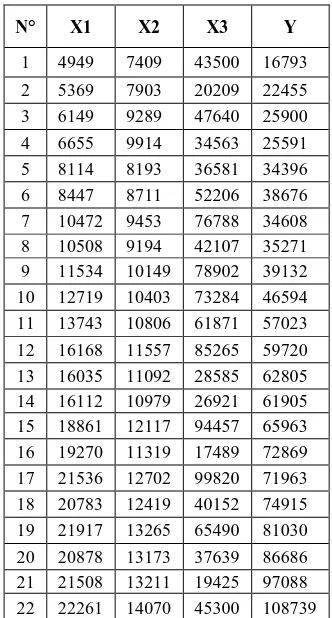
The study is based on a data set used to predict future sales of a product (Y) based on advertising spending (X1), promotional expenses (X2) and quarterly sales of its main competitor (X3).

[image:3.595.49.290.427.584.2]

For this we have 22 observations of three sets of inputs and output series (Table 2).

Table 2. Data set for causal model based MLP

N° X1 X2 X3 Y

1 4949 7409 43500 16793 2 5369 7903 20209 22455 3 6149 9289 47640 25900 4 6655 9914 34563 25591 5 8114 8193 36581 34396 6 8447 8711 52206 38676 7 10472 9453 76788 34608 8 10508 9194 42107 35271 9 11534 10149 78902 39132 10 12719 10403 73284 46594 11 13743 10806 61871 57023 12 16168 11557 85265 59720 13 16035 11092 28585 62805 14 16112 10979 26921 61905 15 18861 12117 94457 65963 16 19270 11319 17489 72869 17 21536 12702 99820 71963 18 20783 12419 40152 74915 19 21917 13265 65490 81030 20 20878 13173 37639 86686 21 21508 13211 19425 97088 22 22261 14070 45300 108739

4.1

Causal model

Neural Network Toolbox provides a complete environment to design, train, visualize, and simulate neural networks. For the causal model we use the function newff to create a feed forward neural network. The Levenberg-Marquardt back propagation algorithme is implemented. “trainlm” is a network training function that updates weights according to Levenberg-Marquardt optimization (Anandhi V. 2012).

Fig.5 Causal Forecast Model Plot Regression

m

Y

5

ˆ



m

Y

Fig.4 Multilayer perceptron for time series forecasting model.

1



m

Y

4



m

Y

. .

.

.

.

. .

.

.

[image:3.595.315.535.530.750.2]

Fig.6 Neural network training for causal forecast model

The figure below compares the results obtained for different architectures integrating three, five and seven neurons in the hidden layer.

Fig.7 Selection of the number of neurons in the hidden layer

We can easily conclude that a network with five neurons in the hidden layer gives very satisfactory results.

4.2

Time series forecasting model

For the neural network training method, we try three algorithms to improve network performance:

- The back-propagation (BP) algorithm: It is a gradient steepest descent method, implemented with traingd function in MATLAB toolbox.

- Gradient descent with adaptive learning rate back-propagation (BPA): traingda function in MATLAB toolbox. - Levenberg-Marquardt back-propagation (LM) : trainlm

function in MATLAB toolbox.

Fig.8 Plot Regression for time series forecast model with BP training algorithm

Fig.10 Plot Regression for time series forecast model with LM training algorithm

The plot regression for the three training algorithms in last figures shown that with the same topology, LM algorithm gives better solution then those found using BP or BPA algorithms.

BP algotithm is the most popular method in training neural networks, however it has a low training efficiency because of its slow convergence: it has a tendency for oscillation (Wilamowski B. M. 2011). To overcome this deficiency, the BPA algorithm uses dynamic learning rate to increase the training speed of BP. However even if the BPA algorithm uses a dynamic learning coefficient, its performance remains less lower than LM, which takes as propagation algorithm a second order function. In fact the LM algorithm can estimate the learning rate in each direction of the gradient using Hussian matrix (Wilamowski B. M., Yu H. 2010).

Fig.11 Demand forecasting with time series model based on neural network

4.3

Comparison between time series

forecasting model and causal model

With the selection of appropriate parameters such as the number of neurons in each layer and selection of the best back-propagation algorithm, the two neural models: time series and causal method, give very similar and satisfactory results

.

Fig.12 MLP forecasting models : time series model and causal model

However, if we take into consideration the cost of the prediction method, the time series model will be chosen since it takes into consideration only the history of the variable to predict. In fact, for a causal model, the collection of predictors is often expensive and can be a source of error in case of erroneous values or inappropriate extrapolation.

5.

CONCLUSION

Demand forecasting plays a crucial role in the supply chain of today’s company. Among all forecasting methods, neural networks models are capable of delivering the best results if they are properly configured. Two approaches based on multilayer perceptron have been developed to predict demand: time series model and causal methods. The best training algorithm is the Levenberg-Marquardt back-propagation algorithm. The number of hidden layers and the number of neurons in each layer depends on the chosen method and case study. With a judicious choice of the architecture and parameters of the neural network, both approaches have yielded good results. However, the cost of the prediction method parameter allows us to prefer the time series model since we have the same results at a lower cost.

6.

REFERENCES

[1] Kesten C. Green, J. Scott Armstrong 2012. Demand Forecasting: Evidence-based Methods. https://marketing.wharton.upenn.edu/profile/226/printFri endly.

42 Bangkok Port. The Asian Journal of Shipping and

Logistics, Vol. 27, N° 3, pp. 463-482.

[3] Armstrong, J. S. 2012 , Illusions in Regression Analysis, International Journal of Forecasting, Vol.28, p 689 - 694. [4] Chase, Charles W., Jr., 1997. “Integrating Market

Response Models in Sales Forecasting.” The Journal of Business Forecasting. Spring: 2, 27.

[5] Chen, K.Y. 2011. Combining linear and nonlinear model in forecasting tourism demand. Expert Systems with Applications, Vol.38, p 10368–10376.

[6] Mitrea, C. A., Lee, C. K. M., WuZ. 2009. A Comparison between Neural Networks and Traditional Forecasting Methods: A Case Study”. International Journal of Engineering Business Management, Vol. 1, No. 2, p 19-24.

[7] Daniel Ortiz-Arroyo, Morten K. Skov and Quang Huynh, “Accurate Electricity Load Forecasting With Artificial Neural Networks” , Proceedings of the 2005 International Conference on Computational Intelligence for Modelling, Control and Automation, and International Conference on Intelligent Agents, Web Technologies and Internet Commerce (CIMCAIAWTIC’05) , 2005

[8] Wilamowski B. M. 2011. Neural Network Architectures. Industrial Electronics Handbook, vol. 5 – Intelligent Systems, 2nd Edition, chapter 6, pp. 6-1 to 6-17, CRC Press.

[9] Zhang G., Patuwo, B. E., Hu, M.Y. 1998. Forecasting with artificial neural networks : The state of the art. International Journal of Forecasting.Vol.14, , p 35–62. [10]Norizan M., Maizah H. A., Suhartono, Wan M. A. 2012.

Forecasting Short Term Load Demand Using Multilayer Feed-forward (MLFF) Neural Network Model. Applied Mathematical Sciences, Vol. 6, no. 108, p. 5359 - 5368 [11]Anandhi V., ManickaChezian R., ParthibanK.T. 2012

Forecast of Demand and Supply of Pulpwood using Artificial Neural Network. International Journal of Computer Science and Telecommunications, Vol.3, Issue 6, June, pp. 35-38

[12]Wilamowski B. M. 2011 Neural Networks Learning. Industrial Electronics Handbook, vol. 5 – Intelligent Systems, 2nd _{Edition, chapter 11, pp. 11-1 to 11-18, CRC}

Press.