Estimation of Ready Queue Processing Time using Efficient Factor Type Estimator (E F T) in Multiprocessor Environment

(1)

Estimation of Ready Queue Processing Time using

Efficient Factor Type Estimator (E-F-T) in Multiprocessor

Environment

ABSTRACT

The ready queue processing time estimation problem appears when many processes remain in the ready queue after the sudden failure. The system manager has to decide immediately how much further time is required to process remaining jobs in the ready queue. In lottery scheduling, this prediction is possible with the help of sampling techniques. Ratio method, existing in literature of sampling, was previously used by authors to predict the time required provided highly correlated source of auxiliary information is available and used.

This paper suggests two new estimation methods which are compared in terms of estimating the total processing time. Under large sample approximation, the bias and m.s.e of proposed estimators have been obtained in the set up of random sampling applicable to lottery scheduling. Performance of both is compared in terms of mean squared error. The confidence intervals are calculated for the estimate and they provide strong numerical support to the theoretical findings.

Keywords

Lottery Scheduling, Efficient-Factor-Type Estimator, Bias, Mean Squared Error (M.S.E), Variance, Confidence Intervals.

1. INTRODUCTION

Suppose there are k processors in a multiprocessor and multi-user environment and a large number of processes, say N, are in a waiting queue. The CPU scheduler adopts lottery scheduling procedure to choose randomly any n processes from the waiting queue (n<N) and allocates to k processors (k<N) in sequential manner. Lottery scheduling is different from basic scheduling algorithm where each process is allocated a number of lottery tickets determining the possibility of process when to use the CPU. At each schedule point, a lottery is held and the process in the ready queue with the winning ticket gets the CPU utilization. Unlike priority scheduling, every job has equal chance of being represented to the processors. Lottery scheduling does not suffer from starvation.

A technical problem appears when N is very large, and because of the congestion in processing occurs, many processes have to wait until they are called in random manner. If all of sudden the system collapses due to failure of power supply or maintenance problem, technical faults or any other unavoidable reasons, the system manager has to look for backup management. His problem at this juncture is to know how much time requires further for finishing up the remaining processes. These

predictions are uncertain and require probability mechanism to resolve. This paper takes such problem and presents two estimation methods for predicting the possible time interval required for processing the remaining jobs.

Shukla and Jain [12] discussed multiprocessor environment, for usual lottery scheduling procedures in order to obtain ready queue time estimate. A method of estimation is suggested by authors and they computed the predicted time intervals. Shukla et al. [8] studied similar problem using systematic lottery scheduling scheme in order to improve upon the prediction of ready queue processing time. Shukla et al. [11] discussed similar problem when processes are grouped according to some criteria in different queues. Shukla et al. [10] introduced size based priority scheme for the ready queue time length prediction and have shown that it is better than usual lottery scheduling in terms of confidence interval for estimates. This paper present E-F-T estimation method for such estimation and compares the two estimation procedures.

2. A REVIEW

Cochran [2] contains an introduction to the methods of sampling theory with application over multiple data. David [3] extended lottery scheduling, a proportional share resource management algorithm to provide the performance assurance present in traditional non real time process scheduler. Dynamic tickets were incorporated into a lottery scheduler to improve the interactive response time and to reduce kernel lock contention. Raz et al. [4] presented procedure of deciding priorities among jobs by maintaining fairness in selection procedure. Shukla and Jain [7] [9] tackled Markov Chain based study of transitions in multilevel queue scheduling. Shukla and Jain [13] performed analysis of thread scheduling and Deficit Round Robin Alternated (DRRA) scheduling algorithm using Markov Chain Model approach. Shukla and Jain [5] suggested a stochastic model for evaluating the reaching probabilities of message flow in space-division switches. Shukla, Jain and Ojha [6] performed a task of analysis of multilevel queue scheduling with the effect of data model approach. Waldspurger [1] proposed that lottery scheduling ticket/currency framework can accommodate scheduling mechanism other than the probabilistic lottery algorithm and discussed the proportional share resource management technique. Singh and Shukla [14] discussed a family of Factor-type ratio estimator for existing population mean. In another contribution Singh and Shukla [15] derived Efficient factor type estimator for estimating the same population parameter.

1

D. Shukla

Deptt. of Mathematics and Statistics

Dr.H.S.Gour Central University

Sagar, (M.P), INDIA

2

Anjali Jain

Deptt. of Computer Science and

Applications

(2)

Yiping [22] developed a queuing theory model to predict system behavior and CPU queue length in Microsoft NT, Windows 2000 and derived fair share scheduling which guarantees application performance by explicitly allocating share of system resources among competing workloads. Some other useful contributions are [16], [17], [18], [19], [20], [21].

3. PROBLEM DEFINITION

It is common and well known idea that often the more input information provides better prediction subject to condition if information is related. Based on this thought the efficient factor type estimation technique has been introduced in order to get more precise confidence intervals compared due to Shukla et al. [14].

4. PROCESSOR STRUCTURE AND

NOTATIONS

Let

Q

1

,

Q

2

,

Q

3

...

.

Q

kbe

k

processors who receive intake from the ready queue containing

P

1

,

P

2

,

P

3

...

.

P

N processes

(n<N). Processes are in long, medium and short term scheduling waiting queues prepared for transferring to ready queue. When a process is blocked or suspended, it is back to respective queue. The figure 1 shows the diagram of scheduling process structured with k processors.

Let;

N: - Total processes in the system.

n:- Sample size of randomly selected processes. f:- Sampling fraction.

i

Y

: - CPU burst time of each ith process



i



1 ,

2 ,

3 ...

N



.

i

X

: - Value of ith auxiliary variable like size of process or process priority or processes response time (time interval between arrival and processor entering).





 N

i i

Y N Y

1 1

: - The mean of CPU burst time of Nprocesses in the ready queue.





N i

i

X N X

1 1

: - The mean of size of Nprocesses in the ready queue.

Y S

C_Y  Y _{: - Coefficient of varation for population parameter Y.}

X S

C X

X  : - Coefficient of variation for population parameter X.

Y X S C XY

XY  : - Coefficient of variation due to X and Y.

4.1 Modified

Multiprocessor

Lottery

Scheduling

[As Shukla, Jain and Chouwdhary[13])

Step I: When a process enters into ready queue, it is allotted a

random number (in specified range).

Step II: Each processor

Q

1

,

Q

2

,

Q

3

...

.

Q

K generates unique

and uncommon random number in similar specified range stated in Step I.

Step III: Matching of both random numbers takes place

between process and processor. If both random numbers are same for a process in ready queue, it is assigned to that processor.

Step IV: Processor either blocks or processes the job. It selects

another process by random manner.

Step V: After when one job processed completely or partially

processors generate time consumed in processing as

y

i(Time

(3)

5. ESTIMATION OF READY QUEUE

PROCESSING TIME (as [12])

We know Ratio estimator:yr yX/x, where y,xare sample

means and Xis population mean.

 

y YPV S



V





B k 02 … (1)

 



02 11



2 2

20 P S V 2PSV

V Y y

M _k    _... (2)

In above expressions





 





/ ; , 0

Ey Y x X Y X Y X

Vij i j i j …

(3)

Consider following notations;



1



2



;

 d d

A





1 



4 

;



d

B



2



3



4



 d d d

C

where d is a constant(0d)_.The class of efficient factor-type estimator proposed by[14] is









   

 

 

  

x C X fB A

x fB X C A y

T_d

...(*)

It gives T1yr,T2yp,T3yaandT4 y[as Shukla et

al.[14]]. The term

y

p

,

y

a are well known product estimator and

Srivenkatramana and Tracy [19] estimator.

The fact that A, B and C can more generally be written



k a1



k a2



;

A  



k

a

₁



k

b

₁



;

B







k a2



k b1



k b2



.

C   

With b2 



a2b1



/2has not defined in Shukla et.al [16]. They

have arbitrarily chosen a11,a22,b14in order to define

(*).However, it has been observed that if structures of A, B, C are not changed different selection ofa1,

a

2,

b

1and



₂ ₁



/2

2 a b

b   do not disturb the properties of the class of estimatorsTd.Changes in the choice of these constants only shift

the origin of d tok.

Blocked/Suspended Long term scheduling Long term scheduling

Medium term scheduling

Ready/ suspended

Ready Queue

Short term scheduling

Medium term scheduling J1

J2

J3

Jn

.

Exit

.

Q3

Q2

Q1

QK

m2 mr mn

… … …

P1 P2 P3

… … …

PN

L1

L2

L3

Ln

[image:3.595.49.545.64.400.2]

.

Figure 1: Ready Queue Processing Under Lottery Scheduling

(4)

We define here the following one-parameter family of T

F

E  estimators:









_         s s k x C X fB A x fB X C A y

T … (4)









               ) ( ) ( x X Cs X C fB A x X fBs X C fB A y

T_k …

(5) Where



s



X x

s

xs 1 ;sn/



Nn



,0s1/2and

C B

A, , andf have same meaning as in (4).

5.1 Performance Measures of

Tk

[As per [14]]

Taking large sample approximations, yY



1e1



and



1 e2



X

x  such that



ij



j i_e _V

e

E ₁ ₂  _, we get

 



 

_



_

                      2 2 1 1 Cse C fB A fBse C fB A e E Y T

E _k …

(6)

As it is obvious that

1

2 _

  fB C A

Cse

... (7)

for all choices of A, B and C, the bias is given by









YPV SV T

Bias( _k) ₀₂ ... (8)

Similarly the expression for m.s.e given by



02 11



2 2 20 2 ) ( .

.SET YV P S V PSV

M _k    _... (9)

.

WhereP

  

fBs / AfBC



and



Cs/



AfBC



.

5.2 Suggested Estimators

UsingShukla et al. [14], we suggest two estimators as below

Atd5, we choose one estimator in class

T

kmarked as TA





          s s A x X f x f X y T 6 4 12 4 18 ... (10)

 

                 f s V s V f fs Y T Bias A 4 18 6 4 18 6 4

02 ...

(11)                          

 02 11

2 2 20 2 4 18 6 4 2 4 18 6 4 ) ( . . sV f fs V s f fs V Y T E S M _A

Similarly at d6, we choose one estimator from class

T

kmarked as

B T





_        s s B x X f x f X y T 24 10 20 10 44 ... (13)

 

                 f s V s V f fs Y T Bias _B 10 44 24 10 44 24 10

02 ...

(14)                          

 02 11

2 2 20 2 10 44 24 10 2 10 44 24 10 ) ( . . sV f fs V s f fs V Y T E S M _B ... (15)

Wheresn/(Nn)

The 95% confidence interval of the estimate using

T

A and

T

B

are:

 

] 0.95 [ 2 , 1    A n

A t V T

T

P  ... (16)

 

] 0.95 [ 2 , 1    B n

B t V T

T

P _ _... (17)

Where

 



 



 

2





A A

A MT BT

T

V   ... (18)

 



 



 

2





B B

B MT BT

T

V   ...

(19)

More explicitly, one can write 95% confidence intervals for mean estimation

 

] 0.95 [ 2 , 1 2 ,

1    



 A A n A

n

A t V T Y T t V T

T

P _ _

 

] 0.95 [ 2 , 1 2 ,

1    



 B B n B

n

B t V T Y T t VT

T

P _ _

where 2 , 1  n

t _{is t-value at (n-1) degree of freedom and at}



_level

of significance and where

T

A,

T

B are the sample based

estimates of population parameter Y . These estimates

T

A,

B

T

are predictors for average time required to complete a process by a processor. Suppose out of Nprocesses, n are processed (n<N) and remaining (N-n) are still in the system when sudden collapse occurs. Then the

predicted total time required for remaining jobs is; where

, 63 . 5362

X Y73.23.





A

A N n T

t   ₍₂₀₎





B

B N n T

(5)

6. NUMERICAL ANALYSIS

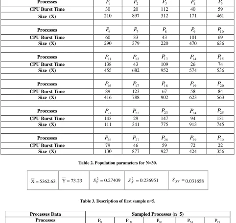
Consider 30 processes in ready queue at a time whose size measure X is also given in terms of bytes. If we assume that all

the processes are processed completely in the ready queue, the CPU burst time Y is mentioned against them.

Table 1. Data of Ready Queue

Processes

P

₁

P

₂

P

3

P

4

P

5

CPU Burst Time

30

20

112

40

59 Size (X)

210

897

312

171

461 Processes

P

6

P

7

P

8

P

9

P

10

CPU Burst Time

60

33

43

101

69 Size (X)

290

379

220

470

636 Processes

P

₁₁

P

12

P

13

P

14

P

15

CPU Burst Time

138

43

109

26

74 Size (X)

455

682

952

574

536 Processes

P

16

P

17

P

18

P

19

P

20

CPU Burst Time

89

123

67

58

84 Size (X)

416

788

902

623

563 Processes

P

₂₁

P

22

P

23

P

24

P

25

CPU Burst Time

143

29

147

94

131 Size (X)

111

341

775

913

745 Processes

P

26

P

27

P

28

P

29

P

30

CPU Burst Time

79

46

59

72

22 Size (X)

130

877

927

424

356

[image:5.595.57.540.144.601.2]

Table 2. Population parameters for N=30.

Table 3. Description of first sample n=5.

Table 4. Population Parameters for first sample( n=5). 63

. 5362

X Y73.23 S_Y2 0.27409 S_X2 0.236951 SXY 

_0.031658

Processes Data

Sampled Processes (n=5)

Processes

P₉ P₁₈ P₃₀ P₂₄ P₁₃

CPU Burst Time (Y

i

)

101

67

22

94

109 Processes Size( X

i

)

470

902

356

913

952

(6)

Table 5. Bias and MSE and confidence interval of

T

Aand

T

Bestimators (When n=5).

Table 6. Description of second sample n=10.

Table 7. Population Parameters for second sample (n=10).

T

Aand

T

Table 9. Description of third sample n=15. )

(T_A

Bias

-0.0115

Bias(T_B)

-0.0126

) ( . .SET_A

M

242.8404

M.S.E(T_B)

241.9289

)

(

T

A

Var

242.8403

Var

(

T

B

)

241.9288

Estimated Confidence Interval lengths

Estimate

(

T

_A

)

95 % Confidence Intervals for

)

(

T

_A

Estimate

)

(

T

_B

95% Confidence Intervals for

)

(

T

_B

71.18 (28.90-115.42)

70.50 (28.98-115.33)

Processes Parameters

Sampled Processes (n=10)

Processes

P₂₀

P

₂₇ P11 P1 P22 P15 P23 P5 P10 P29

CPU Burst Time (Y

i

)

84

40

138

30

29

74

147

59

69

72 Processes Size (X

i

)

563

171

455

210

341

536

775

461

636

424 N=30

n=10

f=0.3333

V0.13361

V

₀₂



0 .015797

V₂₀0.018273 V110.002111

) (T_A

Bias

-0.0047

Bias(T_B)

-0.001

) ( . .SETA

M

96.7872

M.S.E(TB)

96.4893

)

(

T

_A

Var

96.7871

Var

(

T

_B

)

96.4892

Estimated Confidence Interval lengths

Estimate

(

T

A

)

95% Confidence Intervals for

)

(

T

_A

Estimate

)

(

T

_B

95% Confidence Intervals for

)

(

T

_B

147.41 (123.82-168.33)

143.46 (123.86-168.30)

Processes

Data

Sampled Processes( n=15)

Processes

P₁₅ P₂₃ P₅ P₁₀ P₂₉ P₃₀ P₆ P₁₇ P₂₅ P₁₅ P₂₀

P

₂₇ P11 P1 P22

CPU

Burst

Time (Y

i

)

74

147

59

69

72

22

60

123

131

74

84

40

138

30

29 Processes

Size(X

i

)

(7)

[image:7.595.60.531.102.147.2]

Table 10.Population Parameters for third sample (n=15).

T

Aand

T

7. CONCLUSION

Two estimators

T

Aand

T

B_{suggested for estimation of average}

ready queue remaining time. The estimate by

T

A_{= 71.18 while} B

T

_{= 70.50 (when n=5). Both are close to true value. The M.S.E}

of

T

B_{(=241.93) is lesser to the M.S.E of}

T

A_{(=242.84) for n=5.} B

T

_{is uniformly efficient over}

T

_A_{for all n=5, 10 and 15 due to}

lower M.S.E. The true values of CPU burst time lies within the range of confidence interval. It is recommended to prefer

B

T

over

T

A_{in setup of lottery scheduling for estimation}

purpose.

8. REFERENCES

[1] Carl A. Waldspurger and William E. Weihl 1994. Lottery Scheduling a flexible proportional-share resource management. In: Proceedings of the 1st USENIX Symposium on Operating Systems Design and Implementation (OSDI), pp.1-11.

[2] Cochran 2005. Sampling Technique, Wiley Eastern Publication, New Delhi.

[3] David Petro, Garth A. Gibson and John W. Milford 1999. Implementing Lottery Scheduling: Matching the specializations in Traditional Schedulers. In: Proceedings of the USENIX Annual Technical Conference USA, pp.66-80.

[4] Raz, D., B. Itzahak and Levy H. 2004. Classes, Priorities and Fairness in Queuing Systems, Research report, Rutgers University.

[5] Shukla D., Jain, S. 2010. A Stochastic Model Approach for Reaching Probabilities of Message Flow in Space-Division Switches. International Journal of Computer Networks, Vol. 2, Issue 2, pp. 140-151.

[6] Shukla, D, Jain, Saurabh and Ojha, S. 2010. Effect of Data Model Approach for the Analysis of Multi-Level Queue Scheduling, International Journal of Advanced Networking and Applications, Vol. 2 Issue 1, pp. 419-427.

[7] Shukla, D. and Jain, S. 2007. Deadlock state study in security based multilevel queue scheduling scheme in operating system. In: Proceedings of National Conference on Network Security and Management, NCNSM-07, pp. 166-175.

[8] Shukla, D., Jain, A. 2010. Estimation of ready queue processing time under SL scheduling scheme in multiprocessor environment. International Journal of Computer Science and Security (IJCSS), Vol. 4(1), pp. 74-81.

[9] Shukla,D. and Jain, S. 2009. Analysis of Thread scheduling with multiple processors under a Markov chain model, Journal of Computer Science, Vol. 3 , Issue 5, pp. 78-86. [10]Shukla,D., Jain, A. 2011. Analysis of Ready Queue

Processing Time under PPS-LS and SRS-LS scheme in Multiprocessing Environment. GESJ: Computer Science and Telecommunication, 6(26), pp. 99.

[11]Shukla,D., Jain, Anjali and Choduary, A. 2010. Estimation of ready queue processing time under Usual Group Lottery Scheduling (GLS) in Multiprocessor Environment. International Journal of Computer and Applications (IJCA), Vol. 8, No. 14, pp. 39-45.

[12]Shukla,D., Jain, Anjali and Choduary, A. 2011. Estimation of ready queue processing time under Usual Lottery Scheduling (ULS) in Multiprocessor Environment. Journal of Applied Computer Science and Mathematics (JACSM), Vol. 11, No 11, pp.58-63.

[13]Shukla,D., Jain, Saurabh and Singh S. 2008. A Markov chain model for Deficit Round Robin Alternated (DRRA) scheduling algorithm. In: Proceedings of the International Conference on Mathematics and Computer Science, ICMCS-08, pp. 52-61.

N=30

n=15

f=0.5

V0.13361

V

₀₂



0 .007989

V₂₀0.009136 V110.001055

) (T_A

Bias

-0.0017

Bias(T_B)

-0.00261

) ( . .SE T_A

M

48.32569

M.S.E(T_B)

48.2682

)

(

T

_A

Var

48.32568

Var

(

T

_B

)

48.2681

Estimated Confidence Interval lengths

Estimate

(

T

A

)

95% Confidence Intervals for

)

(

T

_A

Estimate

)

(

T

_B

95% Confidence Intervals for

)

(

T

_B

(8)

[14]Shukla D., Singh V.K., Singh G.N. 2001. On the use of transformation in factor-type estimator, METRON International Journal of Statistics, Vol. XLV, pp. 349-361. [15]Singh V.K., Shukla D. 1992. An efficient one-parameter

family of factor-type estimator in sample surveys, METRON International Journal of Statistics, Vol. XVV, pp.139-159.

[16]Singh V.K., Shukla D. 1987. One parameter family of factor type ratio estimators, METRON International Journal of Statistics, Vol. XLV- N. 1-2, pp. 273-283. [17]Silberschatz, A. and Galvin, P. 1999. Operating System

Concepts, Ed.5, John Wiley and Sons (Asia), Inc.

[18]Singh, Daroga and Choudhary, F.S. 1986. Theory and Analysis of Sample Survey and Designs, Wiley Eastern Limited, New Delhi.

[19]Srivenkataramana, T. 1980. A dual to ratio estimator in sample survey, Biometrika, Vol. 67, pp. 199-204.

[20]Stalling, W. 2004. Operating Systems, Ed.5, Pearson Education, Singapore, Indian Edition, New Delhi. [21]Tanenbaum, A. 2000. Operating system, Ed. 8, Prentice

Hall of India, New Delhi.

[22]Yiping Ding, William Flynn 2000. Interpreting Windows NT Processor Queue Length Measurements. In: Proceedings of the 31st Computer Measurement Group Conference, Vol. 2, pp.759-770.