Learning Rates in Generalized Neuron Model for Short
Term Load Forecasting
Chandragiri Radha
Charan
Assistant Professor, EEE Department,
JNTUH, College of Engineering, Nachupally,
Kondagattu, Jagtyal, Karimnagar (Dist.) Andhra Pradesh, India
K.Srinivas
Assistant Professor EEE Department, JNTUH, College of Engineering, Nachupally,
Kondagattu, Jagtyal, Karimnagar (Dist.) Andhra Pradesh, India
K. Pritam Satsangi
Assistant Professor, Department of Electrical
Engineering,Faculty of Engineering, Dayalbagh
Educational Institute, Dayalbagh, Agra, Uttar
Pradesh, India
ABSTRACT
In this paper, Short Term Load Forecasting (STLF) can be applied using Generalized Neuron Model (GNM) for under sum square error gradient function for different learning rates, with various training epochs and constant leaning rate, by having 30,000 training epochs. The simulation results were the root mean square testing error, maximum testing error, minimum testing error were predicted.
General Terms
Short Term Load Forecasting , Generalized Neuron Model, Sum square error gradient.
Keywords
Sum Squared Error Gradient, Generalized Neuron Model, Short Term Load Forecasting.
1.
INTRODUCTION
Short Term Load Forecasting (STLF) is done from an hour to a week which is required for control, unit commitment, security assessment, optimum planning of power generation etc. Different methods such as general exponential smoothing, Kalman filter, multiple regressions, Auto Regressive Moving Average(ARMA) , stochastic time series methods.
In-order to decrease the complexity, decrease the computation time, artificial technique has been suggested such as artificial neural network fuzzy logic, knowledge based systems are used.
The deterministic models provide only the forecast values, not a measure for the forecasting error. The stochastic models provide the forecast as the expectation of the identified stochastic process. They allow calculations on statistical properties of the forecasting error. Regression models are among the oldest methods suggested for load forecasting which are quite insensitive to occasional disturbances in the measurements.
The stochastic time series models have many attractive features. The properties of the model are easy to calculate. The model identification is also relatively easy. Moreover, the estimation of the model parameters is quite straightforward, and the implementation is not difficult.
The weakness in the stochastic models is in the adaptability. In reality, the load behavior can change quite quickly at certain parts of the year. While in ARMA models the forecast
values, the model cannot adapt to the new conditions very quickly, even if model parameters are estimated recursively.
If the load behavior is abnormal on a certain day, this deviation from the normal conditions will be reflected in the forecasts into the future. A possible solution to the problem is to replace the abnormal load values in the load history by the corresponding forecast values.
In order to improve the accuracy of model, better modeling result, include the feature of adaptivity, an artificial neural network (ANN) has been used for STLF. But the drawback of ANN model is the requirement of large training time which depends on size of training file, type of ANN, error functions, learning algorithms, hidden nodes. Chandragiri Radha Charan, Manmohan has proposed that the sum square error gradient by applying STLF with the help of generalized neuron model decreases the non adaptive load and adaptive load with weather parameters.
2.
GENERALIZED NEURON MODEL
O
PKOutput
A2
A1
∑
f1
f2
f3
.
.
.
.
fn
X
1X
2
[image:2.595.60.274.162.506.2]X
nInputs
Fig. 1. Generalized Neuron Model
OPK
∑
XOP
XOB
f1out1
f2out1 f1
f2
fn
f1
f2
fn X1
X2
X3
Xi
∑Wsixi
Wpixi
wfs1
wfs2
wfsn
wfp1
wfp2
wfpn
wfs1
wfs2
wfsn
wfp1
wfp2
wfpn
π
ws1
ws2
ws3
wp1
wp2
wp3
wpi
fnout1
f1out2
f2out2
fnout2
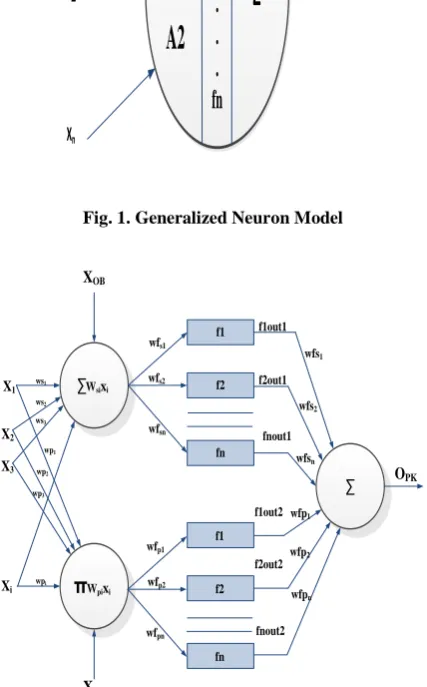
Fig.2. Structure of Generalized Neuron Model
The complexity of GNM is less as compared to multi layered ANN. The flexibility of GNM has been improved by using more number of activation functions and aggregation functions.
In this the model of Fig.1.GNM, contains sigmoid, gaussian, straight line activation functions, with two aggregation functions summation (∑), product (π).The summation and product of an aggregation function have been incorporated and aggregated output passes through non-linear activation function. In Fig.2. , the output of generalized neuron is
1 1 1 1 2 1 1 2 ... 1 1
1 2 1 1 2 2 1 2 ... 2 1 (1)
Opk f out w s f out w s fnout w sn
f out w p f out w p fnout w pn
Here f1out1, f2out1,…. ,fnout1 are outputs of activation functions f1,f2,…,fn related to aggregation function ∑, and f1out2, f2out2, fnout2 are outputs of activation functions f1,f2,…,fn related to π. Output of activation function f1 for aggregation function, f1out1=f1(ws1 sumsigma).Output for activation functions f1 for aggregation function of , f1out2= f1(wfp1product)
3.
DATA FOR STLF UNDER GNM
3.1
Normalized Value for data
Data for the short term load forecasting has been taken from Department of Electricity and water supply, Dayalbagh and Dayalbagh science museum, Agra, India. Different types of conditions have been considered which are mentioned below as different types. The data consists of load of different weeks, weather conditions (maximum temperature, minimum temperature and humidity) have been considered for the month of January 2003. Normalization value:
min
[(
max
min
) * (
)]
(
min
)
max
min
L
L
Y
Y
Y
L
L
(2)
where: Ymax=0.9, Ymin=0.1, L= values of variables, L min= minimum value in that set, Lmax= maximum value in that set
3.2
Sum Square Error Gradient Function
The mathematical expressions were given below. The mathematical expression for the sum squared error gradient
function is
E
sum D
((
Opk
) *
opk
Wsi
Wsi
(3)where E=change in error, Wsi= change in weights, opk= actual output, opk= change in output ,D = desired output.
[image:2.595.48.548.622.758.2]3.3
Data for STLF
Table 3: I, Ii, Iii Weeks Load, Average Maximum Temperature, Average Minimum Temperature, Average Humidity As Inputs And Iv Week Load As Output
First week load
Second week load
Third week load Average maximum temperature
Average minimum temperature
Average humidity
Fourth week load
2196 2295.6 2014.8 10.16 5.66 90 2548.8
2678.4 2286 3087.6 10.5 6.33 90 2560.8
2887.6 2458.8 2618.4 12.5 5.83 85.6 2800.8
2263.2 2479.2 2166 11.5 5.83 87 2461.2
Normalized data
0.17 0.25 0.20 0.55 0.42 0.21 0.54
0.14 0.67 0.25 0.72 0.81 0.90 0.46
0.43 0.68 0.68 0.55 0.90 0.35 0.10
0.31 0.90 0.10 0.32 0.10 0.90 0.64
0.10 0.10 0.09 0.10 0.33 0.64 0.63
0.65 0.10 0.90 0.21 0.66 0.47 0.65
0.90 0.23 0.54 0.90 0.42 0.10 0.90
4.
RESULTS OF STLF UNDER GNM
By applying GNM, STLF problem can be done using learning rates, in different epochs and at constant epoch. The root mean square testing error, maximum testing error, minimum testing error can be reduced. The result is being provided by keeping momentum rate, α = 0.95, gain scale factor = 1.0, all initial weights = 0.95.
4.1
By considering different learning
rates,
The consideration of different learning rates, along with different training epochs will lead to various root mean square testing error, maximum testing error, minimum testing error
4.1.1
Case 1
TABLE 4: Training Epochs Versus Learning Rate - I
Training epoch
Learning Rate,
Result
1-8000 0.0003 Root mean square testing error =2.133×10⁻⁴ Maximum testing error=
2.7325×10⁻⁴
Minimum testing
error=-3.2884×10⁻⁴ 8001-30000 0.0002
0 0.5 1 1.5 2 2.5 3 x 10⁴ 0
0.5 1 1.5 2 2.5 3
Number of Epochs
S
u
m
S
q
u
a
re
d
E
rr
o
r
Training Results of GNM
1 2 3 4 5 6 7
0.1 0.2 0.3 0.4 0.5 0.6 0.7 0.8 0.9 1
Hours
O
u
tp
u
t
Testing Results of GNM
Actual -GNM-1 *
Graph 5: STLF using GNM for sum sqaured error gradient
4.1.2
Case II
TABLE 6: Training Epochs Versus Learning Rate - II
Training epoch Learning Rate, Result
1-5000 0.0004 Root mean square
0 0.5 1 1.5 2 2.5 3
x 104 0
0.5 1 1.5 2 2.5 3
Number of Epochs
S
u
m
S
q
u
a
re
d
E
rr
o
r
Training Results of GNM
1 2 3 4 5 6 7
0.1 0.2 0.3 0.4 0.5 0.6 0.7 0.8 0.9 1
Hours
O
u
tp
u
t
Testing Results of GNM
Actual -GNM-1 *
Graph 7: STLF using GNM for sum square error gradient
4.1.3
Case III
TABLE 8: Training Epochs Versus Learning Rate - III
Training epoch Learning Rate, Result
1-250 0.0006 Root mean square
testing error = 4.0420×10⁻⁹,
Maximum testing error=5.1181×10⁻⁹ Minimum error = -6.2830×10⁻⁹ 251-1000 0.0005
1001 - 30000 0.0004
0 0.5 1 1.5 2 2.5 3
x 104 0
0.5 1 1.5 2 2.5 3
Number of Epochs
S
u
m
S
q
u
a
re
d
E
rr
o
r
Training Results of GNM
1 2 3 4 5 6 7
0.1 0.2 0.3 0.4 0.5 0.6 0.7 0.8 0.9 1
Hours
O
u
tp
u
t
Testing Results of GNM
Actual -GNM-1 *
Graph 9: STLF using GNM for sum square error gradient
4.1.4
Case IV
TABLE 10: Training Epochs Versus Learning Rate - V
Learning rate, Training epochs Results
0.001 1-30000 Root mean square
testing error = 5.2307×10⁻¹⁵, Maximum testing
Graph 11: GNM for STLF , learning rate, =0.001 under sum square error gradient, momentum factor, α=0.95,gain scale factor=1.0, tolerance=0.002,all initial
weights=0.95,trainibg epochs = 30,000.
5.
CONCLUSIONS
The comparision is made between different learning rate‟s,
with number of training epochs and constant learning rate, at 0.001 with number of training epochs which can be simulated in MATLAB 7.0. The results were produced root mean square testing error = 4.0420×10⁻⁹, maximum testing error=5.1181×10⁻⁹ , minimum error = -6.2830×10⁻⁹ by varying learning rate, number of training epochs. By keeping the learning constant as 0.001 under 30,000 epochs the result obtained is root mean square testing error = 5.2307×10⁻¹⁵, maximum testing error=9.992×10⁻¹⁵, minimum testing error = -5.88475×10⁻¹⁵ minimum. By keeping learning rate as constant will achieve very less error as compared to the variation of learning rate by including adaptivity.
6.
ACKNOWLEDGEMENTS
Our thanks to the Dayalbagh science museum and Dayalbagh water and electricity department, Uttar Pradesh, India
7.
REFERENCES
[1] IEEE Committee Report, „”Load Forecasting Bibliography”, Phase 1, IEEE Trans. on Power Apparatus and Systems, vol. PAS-99, no. 1, 1980, pp.53.
[2] IEEE Committee. Report, “Load Forecasting Bibliography” , Phase 2, IEEE Trans. on Power Apparatus and Systems, vol. PAS- 100, no. 7, 1981, pp3217.
[6] M. T. Hagan, “The Time series Approach to Short Term Load Forecasting”, IEEE Trans. on Power System, vol. 2, no. 3, August 1987, pp.785-791.
[7] F. D. Galiana, “Identification of Stochastic Electric Load Models from Physical Data”, IEEE Trans. on Automatic Control, vol. ac-19, no. 6, December 1974,pp.887-893.
[8] S. D. Rahaman and R.Bhatnagar, “Expert Systems Based Algorithm for Short Term Load Forecasting”, IEEE Trans. on Power Systems, vol. 3, no. 2, May 1988, pp.392-399.
[9] K. L. Ho, “Short Term Load Forecasting Taiwan Power System Using Knowledge Based Expert System” ,IEEE Trans. on Power Systems, vol. 5, no. 4, November 1990, pp.1214-1221.
[10] D. Park, “Electric Load Forecasting Using an Artificial Neural Network”, IEEE Trans. on Power Systems, vol. 6, 1991, pp.442-449.
[11] T. M. Peng, “Advancement in Application of Neural Network for Short Term Load Forecasting”, IEEE Trans. on Power Systems, vol. 7, no. 1, 1992,pp. 250-257.
[12] Man Mohan, D. K. Chaturvedi, A.K. Saxena , P.K.Kalra, “Short Term Load Forecasting by Generalized Neuron Model”, Inst. of Engineers (India), vol. 83, September 2002, pp. 87-91.
[13] D.K. Chaturvedi, M. Mohan, R.K. Singh , P.K. Kalra, “Improved generalized neuron model for short-term load forecasting”, Soft Computing, Springer-Verlag, Heidelberg, vol. 8, no. 1, 2003,pp. 10 -18
[14] Man Mohan, D. K. Chaturvedi , P.K. Kalra , “Development of New Neuron Structure for Short Term Load Forecasting”, Int.J. of Modeling and Simulation, ASME periodicals, 2003,vol. 46, no. 5, pp. 31-52
[15] Cha ndragiri Radha Charan, Manmohan, “Application of Adaptive Learning in Generalized Neuron Model for Short Term Load Forecasting under Error Gradient Functions” 3rd
International Conference on Contemporary Computing, Jaypee Institute of Information Technology and University of Florida, U.S.A., August 9th – 11th, 2010, Springer Verlag (Communications in Computer and Information Science-94, Berlin, Heidelberg), Part I , pp. 508–517
[16] Devendra K. Chaturvedi, Soft Computing Techniques and its Applications in Electrical Engineering, Development of Generalized Neuron and Its Validation: Springer- Verlag Berlin Heidelberg, 2008, pp. 87-122.
8. AUTHORS PROFILE
Chandragiri Radha Charan received the B.Sc Engineering from Electrical Engineering Department from Faculty of Engineering Dayalbagh Educational Institute, Agra, Utttar Pradesh. India, in 2003, the M.Tech. Degree in Engineering Systems from Electrical Engineering Department from Faculty of Engineering Dayalbagh Educational Institute, Agra,Uttar Pradesh, India, in 2007.Currently, he is an Assistant Professor in Electrical and Electronics Engineering Department, Jawaharlal Nehru Technological University Hyderabad College of Engineering Karimanagar. His fields of interest include Soft Computing and Power Systems.
K.Srinivas received the B.E. degree in electrical and electronics engineering from Chithanya Bharathi Institutue of Technology and Science, Hyderabad, Osmania University, Hyderabad, India, in 2002, the M.Tech. Degree in power systems and Power Electronics from the Indian Institute of Technology, Madras, Chennai, in 2005, pursuing Ph.D from Jawaharlal Nehru Technological University Hyderabad. Currently, he is an Assistant Professor in Electrical and Electronics Engineering Department, Jawaharlal Nehru Technological University Hyderabad College of Engineering Karimanagar. His fields of interest include power quality and power-electronics control in power systems.