New Method for the Systematic Determination of the
Model’s Base of Time Varying Delay System
Saïda Bedoui
University of Gabes, TunisiaResearch Unit: Numerical Control of Industrial Processes National Engineering school of Gabes, route de Medenine, B.P
6029 Gabes, Tunisie
Majda Ltaief
University of Gabes, TunisiaResearch Unit: Numerical Control of Industrial Processes National Engineering school of Gabes, route de Medenine, B.P
6029 Gabes, Tunisie
Kamel Abderrahim
University of Gabes, TunisiaResearch Unit: Numerical Control of Industrial Processes National Engineering school of Gabes, route de Medenine, B.P
6029 Gabes, Tunisie
ABSTRACT
In this paper, we propose a new method for the systematic determination of the model's base of time varying delay system. This method based on the construction of the classification data related to the considered system. The number, the orders, the time delay and the parameters of the local models are generated automatically without any knowledge about the full operating range of the process. The parametric identification of the local models is realized by a new recursive algorithm for on line identification of systems with unknown time delay. The proposed algorithm allows simultaneous estimation of time delay and parameters of discrete-time systems. The effectiveness of the new method has been illustrated through simulation.
Keywords
Identification, Time delay system, models’ base, Multimodel approach.
1.
INTRODUCTION
Many process include time delay phenomena in their dynamics (such as aircraft, chemical or process control systems) they arise either as a result of inherent delay in the system, as result due to measurement processes or as an introduction of it in the system for control purpose ( in the identification exercise when a higher order process is approximated by a lower order model). The neglect of its presence may leads to a source of complex behavior [5, 6] (oscillations, instability, and bad performance). That is why; a high number of publications are devoted to time delay identification [14, 22, 21]. We cite the principal one to identify time delay system. One approach based on the approximation of the time delay by a rational transfer function or Pade approximation is proposed in [4] [9]. Such approach requires estimation of more parameters because the order of the approximated system model is increased and an unacceptable approximation error may occur when the system has a large delay.
Another method that identifies the time delay and the system parameters is presented in [15]. This method is based on the minimization of the prediction error identification using the Levenberg-Marquadt optimization method with exact derivatives of the objective function with respect to the adjustable parameters that include the time delay.
A linear filter method is introduced for simultaneous parameter and delay estimation of transfer function models. This method estimates the time delay along other model parameters in an iterative way through simple linear regression [11]. Several methods that require the cross
correlation technology in the signal process to identify the time delay system [1] [17] [20]. The method developed in [18] [19] evolves the identification of time delay and the parameters of a system. It based on the minimization of the error between the process output and the process predictive model output, the variable delay parameter is identified. In a somewhat dual way, another one [3] which suggest an algorithm to recursively update the value of a small delay by inspection of the phase contribution of the real negative zero arising in the corresponding sampled system. The main drawback of this method is that iteration on time delay is required to estimate the parameters and this makes on line implementation difficult. A online algorithm for the estimation of both process parameters and delay where no a priori knowledge of the delay is required is presented in [2]. The algorithm is a modification of any standard recursive parameter estimation algorithms and can be applied easily to any of the well established versions of estimation algorithms (Least-Squares, Instrumental Variables, Maximum likelihood, ect..) and their extensions. It is based on two-step procedure, first assumes that a known time delay and estimates the other transfer parameters, then minimizes the least squares error performance index with respect to the delay value.
Nevertheless, there are few algorithms that address the recursive identification of unknown time varying delay system [19].
In this work, we suggest to exploit the multimodel approach for the representation of time varying delay system [12]. The determination of models’ base is based on numerical data classification. This method does not require any knowledge about the operating range of the system, nor about the variation law of the time delay and the system parameters. Besides, we propose a new recursive algorithm for on line identification of systems with unknown time delay. The proposed algorithm allows simultaneous identification of the time delay and the system parameters.
This paper is organized as follows. In the second section, we expose the method used for the multimodel representation of time delay systems
2.
MULTIMODEL REPRESENTATION
OF TIME VARYING DELAY SYSTEM
2.1
The model's base generation
in estimating the structural by the RDI and the parametric using a new identification algorithm.
2.2
The model’s base generation
This method exploits the data classification method proposed by Chiu [13]. It is divided into two steps, the first is to classify the data set obtained from identification measurements. The second treats the structural and parametric identification exploiting the data relating of each cluster obtained from the classification phase.
Construction of the classification data:
The classification procedure consists to select among a set of data points representing classes that will be centers of classes through a computation of potentials.
The classification data s(k) is obtained by a combination of two terms. The first term focus the classification according to the time delay, whereas, the second term focus the classification according to the parameters of the system. The first term is obtained from maximizing the crosscorrelation function between the input and the outputs increments.
( , ) 1 ( )( ( 1) ( ))
k
j
R k h u j h y j y j
k
(1)
s kd( )max( ( ))R k (2)
The second term is a normalization of the output:
max
( ) ( )
p
y k s k
y
(3)
The data s(k) are calculated by the formulation:
s k( )s kd( ) (1 ) ( )s kp
(4) where α is a ponderation between 0 and 1.
Classification procedure:
Having a classification data set (si, i = 1, ...,N), the classification procedure consists to associate to each datum si a potential Pi given by the following expression:
2
2 1
4
( )
M
i j
i
j a
s s
P e
r
(5) where ra is a positive parameter controlling the decrease ratio of the potential. The potential decreases exponentially as sj is away from si. The first cluster center that we call sc1 is the datum whose potential P∗1 is the maximum.
To avoid selecting the first center sc1 and its neighborhood as other cluster centers, the procedure assigns to each potential Pi the following new value:
2 1 *
1 2
4
( i c )
i i
b
s s
P P P e
r
(6) The parameter rb (rb > 0) must be selected larger than ra to favor the operation related to the selection of the other cluster center completely different from the last one.
Next, we select, as second cluster center sc2 whose modified potential given by the relation (6). As similar, we choose the cth cluster center scc with the maximum potential
*
c
P and modify the potentials as follows:
2 *
2
4
( i cc ) (7)
i i c
b
s s
P P P e
r
However, the selection of centers obeyed at each iteration, the following conditions:
• If *
c
P > ε1 P1*, the selection is permitted.
• If *
c
P < ε2
* 1
P , the selection is completed. • If ε2P1* ≤
*
c
P ≤ ε1P1* and if: *
* 1
1 , 1,..., 1 (8)
cc ci c
a
Min s s P
i c
r P
where ε1 and ε2 are two positive parameters (ε1 > ε2) introduced by Chiu, scc is the current center and sc1,sc2,..., sc(c−1) are the last selected ones, the center to be retained corresponds, in this case, to the maximum value of the potentials after rejecting the current value *
c
P .
After the selection of the cluster center, we have a search the elements belonging to each class by a simple computation of distance between si and scc and classify si into the class whose distance is minimum.
Clusters’ modeling:
After the collection of data for each class c (c = 1, ...,N) and assigning the correspond outputs, structural (order of
polynomials ˆ -1 ˆ -1
( , ) ( , )
A k q and B k q
)
and parametric identification must be carried out to elaborate the local model [8]. Each local model can be representing by the following structure:
1 1
( ) ( ) ( ) (9)
a b
n n
c cl c cj c c
l j
y k a y k l b u k j d
Structural identification related to the estimation of the order μc of each model uses the instrumental determinants’ radio test.
Considering the data set related to the cluster c (nc,data), the estimation-procedure of the order μc builds for an order μ (μ = 1, 2...μmax) the information matrixes Qμ and Qμ+1 and evaluate the ratio of the determinants RDI(μ) given by the relation (10) and (11). We maintain as order μc for the cluster c, the value of μ for which the ratio RDI(μ) increases abruptly in first time. Indeed, the Qμ+1 matrix become singular when μ is identified with exact order.
T
1
( )
( 1) ( 1)
( 1) ( 1)
1
( 2) (10)
( )
( 1) ( )
( )
c
c t
c t
c t
c t c t
n
µ t c t
c
c t
c t c t
t
u k
y k u k
u k u k
Q u k
n
y k µ
u k µ u k µ
k µ
1
det( )
( ) (11) det( )
µ
µ
Q RDI µ
Q
The parametric identification uses a new algorithm for simultaneous identification of time delay system and the system parameters. It exploits the observation vector relating to the same cluster c.
2.3
Generation of the multimodel output
1
( ) ( ) ( ) (12)
N
m c c
c
y k v k y k
Where yc(k) is the elementary output of the model Mc and vc(k) is corresponding validity carried out using the residue approach.
2.4
Validities estimation based on classical
residue approach
The validities of models Mc(c = 1, ...,N) are computed using the residues approach formulated by the relations (13)-(16): ( )r kc y k( )y kc( ) (13) where N is the number of local models [8].
This expression must be normalized to have a residue between 0 and 1:
' 1
( )
( ) (14) ( ) c c N j j r k r k r k
The validity which varies in the contrary sense of the residue, can then be expressed by:
'
( ) 1 ( ) (15)
c c
v k r k
We consider the normalized validities given by:
' ( )
( ) (16) 1 c c v k v k N
3.
PARAMETRIC IDENTIFICATION OF
LOCALMODELS
3.1
The proposed approach
This paragraph proposes an alternative solution for the purpose of online and simultaneous identification of unknown time delay and the system parameters.
Equation (17) can be rewritten as:
y kc( ) ( , )k dccv k( ) (17)
where θc is the parameter vector and ϕc(k, dc) is the observation vector which are defined as:
1 2 1 2
( 1), ( 2), , ( ),
( , )
( 1), , ( )
, , , , , , ,
a b
c c c a
c c
c c c c b
T
c c c cn c c cn
y k y k y k n
k d
u k d u k d n
a a a b b b
(18)
On the hand, the estimated output is described by the following relation:
y kˆ ( ) c ˆ( , k dˆ ˆc) c (19)
where ˆθc and ˆ dc represent the estimated parameter vector and the estimated delay.
Now, let consider the prediction error: ˆ ˆ ˆ ˆ
( ) ( ) -c c( ) ( ) - ( , c c) c
e k y k y k y k k d
(20) This formulation does not admit the unknown time delay in the parameter vector and consequently it is not directly applicable to achieve our objective which is simultaneous identification of the time delay and the parameters of time-varying delay systems.
To overcome this problem, we suggest considering the delay in the vector of parameters to be estimated. Indeed, the new vector, called generalized vector of parameters is given by:
,
c
T
G c dc
Moreover, we propose the use of the negative gradient of the error to obtain an appropriate observation vector which is given by:
ˆ
( ) ˆ (21)
c c G G e
ˆ 1 1 ˆ ˆ ˆ
( ) ( ), c ( )(1 ) (22)
c c
T nb
d T
G c c i c
i
d b q u k i q
Replacing T(ˆ)
c dc
by its expression, we obtain the generalized vector parameters: ˆ ˆ ˆ 1 1 ( 1) ( ) ( 1) ˆ
( ) (23)
( )
ˆ ( )(1 )
c c c b c c T c c a d c G d c b n d i c i y k
y k n
q u k
q u k n
b q u k i q
Where Δu(k) = u(k) − u(k − 1). An estimation ˆ
c
G
of
c
G
is denoted by the minimization of the following criterion [23]:
2 01
( ) (24) 2
k
i
J e i
Then, the partial derivative of the criterion with respect to the generalized vector parameter is:
0 0 ( ) ( ) ( , ) ( ) k k G i i G G
J e i
e i i e i
0 0 ˆ ( , ) ( ) ˆ ˆ ( , ) ( ) c c c kG c c c
i G
k
G c c c
i
J
i y i
i y i
Whereˆ 1 1
ˆ ˆ ( )(1 ) (25)
b c c
n d
c i c
i
d b q u k i q
Then, 0 0ˆ ˆ ˆ
( , ) ( ) ( , ) ˆ
ˆ ˆ ˆ
( , ) ( ) ( , )
c c c
c
c c c
k
T
G G G
i G
k
T
G c G G
i
J
i y i i
i y i i
By canceling the partial derivative of the criterion, we obtain:
1
0 0
ˆ ( ,ˆ ) ( ,ˆ ) ( ,ˆ ) ( ) (26)
c c c c
k k
T
G G G G c
i i
i i i y i
Let, 0 ˆ ˆ( ) ( , ) ( , ) (27)
c c
k
T
G G
i
R k i i
Then
1
0
ˆ ( ) ( ,ˆ ) ( )
c c
k
G G c
i
R k i y i
1 1 0ˆ ( ) ( ,ˆ ) ( ) ( ,ˆ ) ( )
c c c
k
G G c G c
i
R k i y i k y k
1ˆ ( ) ( 1) ( 1) ( , ) ( )
c
G R k R k G k k G y kc
1
ˆ ( ) ( )ˆ ( 1) ( ,ˆ ) ( ,ˆ )ˆ ( 1) ˆ
( , ) ( )
c c c c c
c
T
G G G G G
G c
R k R k k k k k
k y k
So,
1ˆ ˆ ( 1) ( ) ( ,ˆ ) ( ,ˆ )ˆ ( 1) ( ) (28)
c c c c c
T
G G k R k k G k G G k y kc
It follows from (28) that
1
ˆ ˆ ( 1) ( ) ( ,ˆ ) ( ) ˆ
c c c
G G k R k k G y kc c c
We obtain finally:
ˆ( ) ˆ( 1) ( ) ( , ) ( ) (30)
G k G k P k k G e k
1 0 1 ˆ ˆ ( ) ( , ) ( , ) ˆ ˆ
( 1) ( , ) ( , )
c c c c k T G G i T G G
P k i i
R k k k
By using the matrix inversion lemma, we obtain:
ˆ ˆ
( 1) ( , ) ( , ) ( 1)
( ) ( 1) ˆ ˆ (31)
1 ( , ) ( 1) ( , )
c c c c T G G T G G
P k k k P k
P k P k
k P k k
The above approach can be summarized by the following step by step procedure:
Step1: Initialization: set ˆ
c
G
=
0
G
= [0(1,na) 0(1,nb) 0(1,1)] and P=βI(na+nb+1) where β is a scalar and I(na+nb+1)is the identity matrix of size (na+nb+nc+1) and k = 0.
Step2: Increment k and constructing the generalized observation vector (ˆ )
c
G
and the observation vector T(ˆ)
c dc
,
Step3: Estimating the ˆ
c
G
by applying the developed identification method (31, 32, 33):
ˆ ˆ ˆ
( ) ( ) - ( , c c) (c 1) (31)
e k y k k d k
ˆ ˆ
( 1) ( , ) ( , ) ( 1)
( ) ( 1) ˆ ˆ (32)
1 ( , ) ( 1) ( , )
c c c c T G G T G G
P k k k P k
P k P k
k P k k
ˆ ( ) ˆ ( 1) ( ) ( , ) ( ) (33)
c c c
G k G k P k k G e k
Step4: Return to step 2 until k = N where N is the number of input/output data.
3.2
Lemma
For the estimate (27) with the assumption A4, the following proprieties are hold:
P1. ˆ
c
G
is an unbiased estimate of .
c
G
P2. The covariance matrix of ˆ
c
G
is given by:
1 2
0
ˆ ˆ ˆ ˆ
( )( ) ( , ) ( , ) (34)
c c
k
T T
Gc Gc Gc Gc G G
i
E i i
ProofIf we replace the equation (17) in (26), we have:
1
0 0
ˆ ( ,ˆ ) ( ,ˆ ) ( ,ˆ ) ( , ) ( )
c c c c
k k
T
G G G G c c c
i i
i i i i d v i
Then
1 0 0 1 0 0ˆ ( ,ˆ ) ( ,ˆ ) ( ,ˆ ) ( , )
ˆ ˆ ˆ
( , ) ( , ) ( , ) ( )
c c c c
c c c
k k
T
G G G c G c c
i i
k k
T
G G c G
i i
i i i i d
i i i v i
So, 1 0 0ˆ ˆ ( ,ˆ ) ( ,ˆ ) ( ,ˆ ) ( ) (35)
c c c c c
k k
T
G G G G G
i i
E E i i i v i
Since ( ,i ˆGc)is independent of v(i), then:
ˆ ˆ
(36)
c c
G G
E
Which proves (P1).
The first order Taylor series expansion around the real parameter of ˆ
c
G
is given by:
2
2
ˆ
( , ) ( , ) ( , ) ˆ
( ) (37)
ˆ c c c c c
c c
c
G G G
G G
G G
G
J k J k J k
Since ˆ ( , ) 0 ˆ c c G G
J k
, it derives from (37) 1 2 2 1 2 2 ( , ) ( , ) ˆ ˆ ( )( ) ( , ) ( , ) c c
c c c c
c c
c c
c c
G G
T
G G G G
G G
T T
G G
G G
J k J k
J k J k
The second partial derivative of the criterion with respect to the generalized vector parameter is given by:
2 2 2 2 0 ( , ) ( ) ( ) ( ) ( , ) c c
c c c
k G
G i
G G G
J k e i e i
e i i
So, 2 2 2 2 0 ( , ) ( ) ( ) ( , ) ( , ) c c c c c k G T G G i G GJ k e i
e i i i
When k0then,
2
2 0
( )
( ) 0
c k i G e i e i
Hence, an approached of
2 2 ( , ) c c G G
J k
is obtained:
2
2
0
( , )
( , ) ( , ) (38)
Applying the mean value of ( , c) ( , c)
c c
T
G G
G G
J k J k
, we
get:
0
( , ) ( , )
( , ) ( , ) ( ( ) ( ) )
c c
c c
c c
T k
G G T T
G G
i
G G
J k J k
E i i E e i e i
So,
20
( , ) ( , )
( , ) ( , )
c c
c c
c c
T k
G G T
G G
i
G G
J k J k
E i i
Then, we have:
¨ 1 1 ¨ 1
2
0
ˆ ˆ
( )( )
( , ) ˆ ˆ ( , )
( , ) ( , )
c c
c c
c c
T Gc Gc Gc Gc
T k
G T G
G G i
G G
E
J k J k
E i i
Finally, we obtain:
1 2
0
ˆ ˆ ˆ ˆ
( )( ) ( , ) ( , )
c c
k
T T
Gc Gc Gc Gc G G
i
E i i
Which proves (P2).
4.
SIMULATION
4.1
Deterministic case
We consider a discrete non stationary second order system with time varying time delay described by the following equation:
1 2
1 2
( ) ( ) ( 1) ( ) ( 2)
( ) ( 1 - ( )) ( ) ( 2 ( ))
r r
r r
y k a k y k a k y k
b k u k d k b k u k d k
[image:5.595.324.530.132.261.2]The variation laws of the parameters (air(k), bir(k)) and the time delay d(k) are presented in figure 1.
Fig 1. The variation laws of the system parameters
Identification phase:
The system is excited in its full operating range by a pseudo random binary sequence so as to generate the necessary classification data s(k).
Clusters generation
The application of the classification methods leads to two clusters focused on the cluster centers sc1 and sc2 which will
be modeled to form the models’ base. The evolution of the potentials during the classification procedure and the emplacement of the cluster centers are presented in the figure 2.
Fig 2. Evolution of the potentials during the classification procedure and emplacement of the cluster centers
Clusters modeling
[image:5.595.339.518.398.636.2]After obtaining the classes and the corresponding elements, we carry out firstly a structural identification of the obtained models (Mc, c=1,2) realized by the test of the Instrumental Determinant Ration (RDI). Figure 3 shows the order estimation of each cluster.
Fig 3. Evolution of the RDI
[image:5.595.67.268.500.613.2]Table 1. The parameters and the time delay of each model of the base (Deterministic case)
Local models ai bi di
M1 −0.1
0.2
0.3
0.15 2
M2 −0.1565
0.3362
0.4425
0.3612 1
The efficiency of the proposed method can be demonstrated by recourse on figure 1 and table 1.
Validation phase:
A validation of the model base, using a sinusoidal input described by the relation (42), is realized.
0.005
(1 sin( / 20)) 200 ( )
( 200) .
k
e k k
u k
u k else
(42)
Figure 4 shows the evolution of the multimodel output ym(k) and the real system output y(k). It can be seen that the multimodel output ym(k) coincides with the real system output.
Fig 4. Real system’s output y(k) and Multimodel output
ym(k) (Deterministic case).
4.2
Stochastic case
We take again the same system with the same parameters’ and time delay variation law and a signal of noise v(k) is add to the system’s output with signal noise ratio (SNR) is equal to 5.
1 2
1 2
( ) ( ) ( 1) ( ) ( 2)
( ) ( 1 - ( )) ( ) ( 2 ( )) ( )
r r
r r
y k a k y k a k y k
b k u k d k b k u k d k v k
A set of noisy classification data is picked out on the system and are treated following the same steps to generate the models’ base of time delay system.
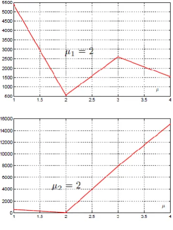
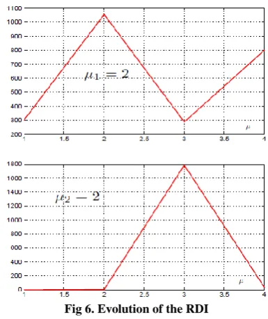
[image:6.595.49.289.96.156.2]In fact the classification procedure yields to two clusters which are modeled by two second order models (see figures 5 and 6) having the parameters and time delay given in table 2.
Fig 5. Evolution of the potentials during the classification procedure and emplacement of the cluster centers
[image:6.595.68.262.308.429.2]Fig 6. Evolution of the RDI
Table 2. The parameters and the time delay of each model of the base (Stochastic case)
Local models ai bi di
M1 0.0752
0.2547
0.0451
0.2061 2
M2 −0.1754
0.4876
0.3583
0.3644 1
[image:6.595.309.551.348.405.2]The same signal of validation u(k) is considered to validate the models base generated from the noisy classification data. The figure 7 presents the evolution of the real system’s output y(k) and multimodel output ym(k). We can see clearly that the multimodel output can describe with precision the real output of the system. The model’s base is valid for the description of the system behavior relatively to one generated in the deterministic case. So, this confirms the robustness of the suggested multimodel representation.
Fig 7. Real system’s output y(k) and Multimodel output
ym(k) (Stochastic case)
5.
CONCLUSION
[image:6.595.332.519.519.633.2] [image:6.595.64.269.622.731.2]generation of the number, the orders, the time delay and the parameters of the local models without any prior knowledge about the operating area of the system. In addition, we have focus, in this paper, on the main issue to consider is the both identification of the time delay and the system parameters. So, we proposed an alternative solution for this aim which consist to consider the time delay in the vector of parameters to be estimated. Moreover, the validation results recorded in this work demonstrate a very satisfactory precision of the modeling using the proposed method.
6.
ACKNOWLEDGEMENTS
This work was supported by the Ministry of the Higher Education and Scientific Research in Tunisia.
7.
REFERENCES
[1] A.B. Rad, W.L. L, K.M. Tsang, 2003, ”Simultaneous on line identification of rational dynamics and time delay: A correlation based approach”, IEEE Transactions on Control Systems Technology, vol. 11, no. 6, pp. 957– 959.
[2] A. Elnaggar, G.A. Dumont, 1990, A.L. Elshafei, ”New method for delay estimation”, Proceeding of 29th Conferenceon Decision and Control, Hawail.
[3] G. Ferretti, C. Maffezzoni, R. Scattolini, , 1991 Recursive estimation of time delay in sampled Systems, Automatica, vol. 27, No. 4, pp. 653-661, Great Britain.
[4] H. Kurz, W. Goedecke, 1981, ”Digital parameter adaptative control of process with unknown dead time”, Automatica, Great Britain, vol.17, no. 1, pp. 245–252. [5] J.P. Richard, 2003,” Time delay systems: an overview of
some recent advances and open problems”, Automatica, vol. 39 , pp. 1667–1694.
[6] Kolmanovskii, V.B. Niculescu, S.I. Gu, K. 1999, ”Delay effects on stability: A survey”, Proceedings of the 38th IEEE Conference on Decision and Control, vol.2, pp. 1993–1998.
[7] M. De la Sen, 2007, Robust adaptive control of linear time delay systems with point time-varying delays via multiestimation, Elsevier, vol. 33, pp. 959–977.
[8] M. Ltaief, K. Abderrahim, R. Ben Abdennour, 2008, ”Contribution to the multimodel approach: Systematic determination of the models’ base and validities estimation”,J Automation and Systems Engineering, vol.2, no. 3.
[9] P.J. Gawthrop, M.T. Nihtila, 1985, Identification of time delays using polynomial identification method, Systems and Control Letters , North-Holland, vol.5, pp. 276–271. [10] Q. G. Wang, Y. Zhang, 2001, Robust identification of
continuous systems with dead time from step responses, Automatica, vol.37, pp. 377–390.
[11] S. Ahmed, B. Huang, S.L. Shah, 2006, Parameter and delay estimation of continuous time models using a linear filter, Automatica, vol.16, pp. 323–331.
[12] S. Bedoui, M. Ltaief, K. Abderrahim, R. Ben Abdennour, 2011,”Representation and control of time delay system: Multimodel approach”. Proceeding of 8th International Multi-Conference On Systems, Signals And Devices, March, Sousse, Tunisia.
[13] S.L. Chiu, 1994,”Fuzzy model identification based on cluster estimation”, Journal of Intelligent and Fuzzy Systems, vol. 2, pp. 267–278.
[14] S.V. Drakunova, W. Perruquettib, J.P. Richard, L.Belkourac, 2006, ”Delay identification in time-delay systems using variable structure observers”, Annual Reviews in Control, vol. 30, no. 2, pp. 143–158.
[15] S.W. Sung, I.B. Lee, 2001, Prediction error identification method for continuous time processes with time delay, Ind. Eng. Chem, vol.40, no.24, pp. 5743– 5751.
[16] T. Zhang, Y. Cui, 2008, A Bilateral Control of Teleoperators Based on Time Delay Identification, IEEE Transactions on Control Systems Technology, China. [17] T. Zhang, Y. Li, 2003, A fuzzy Smith control of
time-varying delay systems based on time delay identification, Proc. of Machine Learning and Cybernetics, vol. 1, pp. 614- 619.
[18] W.Gao, Y.C.Li, G.J.Liu and T. Zhang, 2003, An Adaptive Fuzzy Smith Control of Time-Varying Processes with Dominant and Variable Delay, Proc. of ACC, vol. 1, pp. 220-224.
[19] W. Gao, M. L. Zhou, Y. C. Li, T. Zhang, 2004, An adaptive generalized predictive control of time varying delay System, Proceeding of the second World Conference on Machine Learning and Cybernetics, pp. 878–881, Xi’an, Shanghai.
[20] W.X. Zheng, C.B. Feng, 1990”Identification of stochastic time lag systems in the presence of colored noise”, Automatica, , vol. 26, no. 4, pp. 769–779. [21] Y. Orlov, L. Belkoura, M. Dambrine, J.P. Richard,
2002, ”On identifiability of linear time-delay systems”, IEEE Transactions on Automatic Control, vol.47, no. 8, pp. 1319–1324.
[22] Y. Orlov, L. Belkoura, J.P. Richard, M. Dambrine, 2003, Adaptive identification of linear time-delay systems, International Journal on Robust and Nonlinear Control, vol. 13, no.9, pp. 857–872.