Adaptive Digital Image Filter using Functional Link Artificial Neural Network

Adaptive Digital Image Filter using Functional Link

Artificial Neural Network

Subasish Mohapatra

Institute of Technical Education and Research

Siksha ‘O‘ Anusandhan University

Radha Lath

Institute of Technical Education and Research

Siksha ‘O‘ Anusandhan University

Jyotiprakash Sahoo

Institute of Technical Education and Research

Siksha ‘O‘ Anusandhan University

ABSTRACT

In this paper we have proposed a computationally efficient artificial neural network (ANN) for the purpose of adaptive image filtering. The major drawback of feed forward networks such as multilayer perceptron (MLP) trained with Back Propagation (BP) algorithm is that it requires a large amount of computation time for learning. We propose a single layer functional link ANN (FLANN) in which the need of hidden layer is eliminated by expanding the input pattern by different functional expansions. The novelty of this network is that it requires less computation than that of MLP. We have shown the effectiveness in the problem of filtering an image corrupted with different noises such as additive white Gaussian noise, impulse noise or both of these two, salt & pepper noise, multiplicative noises, random value impulse noise etc. at the time of transmission. To avoid this noise, FLANN based adaptive image filters are used. This can be better utilized in online application. The result is also compared to that of MLP classifier. It is observed that the proposed network is computationally cheap and gives better classification accuracy than that of MLP.

Keywords

Salt &Pepper noise, Gaussian noise, impulse noise, multiplicative noise, MLP, FLANN.

1.

INTRODUCTION

Owing to the imperfections of sensors and communication channels, most images are degraded during the processes of acquisition and transmission. The original images are often contaminated by a mixture of different types of noises. Many applications in the modern digital age are based on images and therefore the resulting achievements must rely on their quality. Image Filtering forms a significant preliminary step in many machine vision tasks, such as object tracking and recognition. A major concern in designing image de-noising models is to preserve important features of image, such as those can be most easily detected by the human visual system, while removing noise. It is important to eliminate the noise automatically and efficiently. Image restoration is historically one of the oldest concerns and still a necessary processing step for many applications. As the field requires higher levels of reliability and efficiency, mathematical image processing has become an important component. So the ultimate goal of restoration technique is to improve accuracy of an image. It is purely an objective process unlike image enhancement, which is a subjective one. Restoration attempts to reconstruct or recover an image that has been degraded by using a prior knowledge of degradation phenomena [1]. Restoration technique may be in spatial domain or it may be in frequency domain. Spatial processing is applicable when the only degradation is additive noise. The Random-noise reduction is carried out in the spatial domain using convolution masks. On the other hand, frequency

domain is found to be idle for reducing periodic noises and for modeling some important degradation such as image blur caused by motion during image acquisition which is difficult to approach in the spatial domain using small masks. In this case frequency domain filters based on various criteria of optimality are the choice of approaches. The word optimality in this context refers strictly to mathematical concept, not to optimal response of the human visual system [1][16].

Several traditional filters have been proposed for restoration of images corrupted by impulsive noise [2].The median filter can be easily designed to suppress non-Gaussian noise and preserve signal structures such as edges and lines. However, when the noise ratio in the contaminated image becomes high, it fails in restoration. For improvement of the accuracy in the standard median filter technique, several methods have been proposed, such as the weighted median filter [3[4][5], which is an extension of the median filter that gives more weight to some values within the window. It emphasizes or de-emphasizes specific input samples, because in most applications, not all samples are equally important.

and selection of training data. Single layer neural network accurately detects the impulse noise of fixed amplitude. However it dose not perform well in case of random value impulse noise. An ANN threshold-filtering scheme is an adaptive filter.

Recently artificial neural network (ANN) has emerged as a powerful learning technique to perform complex tasks in highly nonlinear environment [9]. The advantages of ANN model are due to there ability to learn based on optimization of an appropriate error function and there excellent performance for approximation of nonlinear functions.

As an alternative to the MLP there has been considerable interest in radial basis function (RBF) network [10]. The RBF networks can learn functions with local variations and discontinuities effectively and also possess universal approximation capability. This network represents a function of interest by using members of a family of compactly or locally supported basic functions, among which radially symmetric Gaussian functions, are found to be quite popular. A RBF network has been proposed for effective identification of non-linear dynamic system [10]. But in these networks choosing an appropriate set of RBF centers for effective learning is still a problem. A special case of RBF network where the use of wavelets, not necessarily of radial symmetry, have been proposed in [11].

The functional link artificial neural network (FLANN) by Pao [12] can be used for function approximation and pattern classification with faster convergence and lesser computational complexity than a MLP network. A FLANN using sin and cos function for functional expansion for the problem of nonlinear dynamic system identification has been reported [13].A single layer orthogonal neural network using Legendre polynomials has been reported for static function approximation. Sadegh reported a function basis perceptron network for functional identification and control of nonlinear systems. Linear and nonlinear ARMA model parameter estimation using an ANN with polynomial activation functions for biomedical application has been reported. A FLANN approach using a tensor model for expansion has been applied to thermal dynamic system identification.

In this work we proposed a FLANN structure similar to a Chebyshev polynomial-based unified model ANN [14] and [15] for de-noising in an image corrupted with different noises. Generally a linear node in its output is used in the FLANN structure reported by other researchers.

This paper tries to improve the time complexity involved in training the network, along with minimizing the number of interconnection weights and biases that are used as the network parameters which make it suitable for on-line application in comparison to MLP. This technique is able to approximate linear as well as non linear functions. This is computationally cheap and has small convergence time. It de-noises image more efficiently.

The rest of the paper is organized as follows. Section 2 discusses the proposed works while Section 3 gives the details of the simulation study. Section 4 discusses the summary of simulation & Conclusion. Section 5 discusses the future work.

2.

PROPOSED MODEL

Different type of static filters is used to retrieve images contaminated by different types of noise. In this model, we have designed an adaptive image filter which can restore images contaminated by different types of noises with varying noise density. This filter gives better performance accuracy in

comparision to other static filters like mean, median and random order etc and adaptive filters based on MLP. For functional expansion of the input pattern, we choose the trigonometric and chebyshev polynomial expansions. The primary purpose of this paper is to highlight effectiveness of the FLANN structure in the problem of filtering of image corrupted with different noises. In this paper we briefly describe the architecture and learning algorithm for three types of ANN structures (i.e. Single layer perceptron, MLP and FLANN) used in the study.

2.1

Functional Link Artificial Neural

Network

2.1.1

Mathematical Analysis of FLANN

The learning of an ANN may be considered as approximating or interpolating a continuous, multivariate function f(x) by an approximating function fw(x). in the FLANN a set of basis functions and a fixed number of weight parameters W are used to represent fw(x). With a specific choice of a set of basis functions, the problem is then find the weight parameters W that provides the best possible approximation of f on the set of input-output examples.

2.1.2

Structure of FLANN

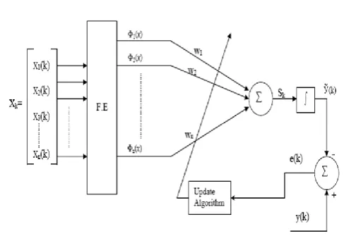
The FLANN, which is initially proposed by Pao [5], is a single layer ANN structure capable of performing complex decision regions by generating nonlinear decision boundaries. In a FLANN the need of hidden layer is removed. In contrast to linear weighting of the input pattern produced by the linear links of a MLP, the functional link acts on an element or the entire pattern itself by generating a set of linearly independent functions. Here the functional expansion block comprises of exponential polynomials. Suppose input to this structure is X=[x1 x2]’. An enhanced pattern obtained by using functional expansion given by X= [1x1T2(x)……x2T2(x2)……] ’.

F.E: - Functional Expansion

Fig.1: Structure of FLANN with a single output

the FLANN becomes simple and has a faster convergence due to its single layer architecture.

Here the proposed network is trained with some reference image and test it in some other image. It is found that the proposed network is able to train at any image given to it and the trained network can be used for cancellation of noise from any other noisy image. Here the performance of the proposed network with that of single layer neural network and MLP network are compared. The primary purpose is to highlight the effectiveness of the proposed simple ANN architecture in the problem of denoising of image corrupted with different noise.

2.1.3 Learning with the FLANN

Referring to figure-2, let there be K number of input-output pattern pairs to be learned by the FLANN. Let the input pattern vector X is of dimension and for ease of understanding, let the output, y be a scalar. Each of the input patterns is passed through a functional expansion block producing a corresponding N-dimensional (N>=n) expanded vector. Detail of the theory on the FLANN may be found in [6].

In this case, the dimension of the weight matrix is of 1 x N and hence, the individual weights are represented by a single subscript. Let w= [w1 w2…..wN] be the weight vector of its FLANN. The linear weighted sum, Sk is passed through the tanh (.) nonlinear function to produce the output Ў (k) with the following relationship:

2.1.4 The Learning Algorithm

Let K number of patterns be applied to the network in a sequence repeatedly. Let the training sequence be denoted by {Xk,Yk} and the weight of the network be W(k), where k is the discrete time index given by k=k+λk, for λ=0,1,2…, and k=0,1,2….,K. At kth instant, the n-dimensional input pattern and the m-dimensional FLANN output are given by

Xk=[x1(k) x2(k)……..xn(k)]T and

Ў(k) = [Ў1 (k) Ў2 (k)…….. Ўm (k)] T respectively. Its corresponding target pattern is represented by Y (k) = [y1 (k) y2 (k)…….. ym (k)]T.

The dimension of input pattern increases from n to N by a basis function Ф given by

Ф (Xk) = [Ф1 (Xk) Ф2 (Xk)…….. ФN (Xk)]T

The (mxN) dimensional weight matrix is given by W(k)=[W1(k)W2(k)……..Wm(k)]T

Where Wj(k) is the weight vector associated with jth output and is given by

Wj (k) = [Wj1 (k) Wj2 (k)……..WjN (k)] The jth output of the FLANN is given by

for j=1, 2, 3….m

Let the corresponding error be denoted by ej (k) =yj (k) - Ўj (k). Using the BP algorithm for single layer, the update rule for all the weights of the FLANN is given by

where W(k)=[W1(k)W2(k)……..Wm(k)]T is the m x N dimensional weight matrix of the FLANN at the kth time instant. δ(k)=[ δ1(k) δ2(k) ……. δm(k)]T, and

[δj (k) = (1- Ўj (k) 2) ej (k)]

2.1.5 Trigonometric Functional Expansion

Here the functional expansion block make use of a functional model comprising of a subset of orthogonal sin and cos basis functions and the original pattern along with its outer products. For example, consider a two dimensional input pattern X=[x1x2] T, the enhanced pattern is obtained by using a trigonometric functions as x'= [x1cos (πx1) sin (πx1) cos (3πx1) sin (3πx1)]. The LMS algorithm, which is used to train the network, becomes very simple because of the absence of any hidden layer.

2.1.6 Chebyshev Expansion

The Chebyshev polynomials [18][19]are a set of orthogonal polynomials defined as the solution to the Chebyshev differential equation and denoted as Tn(x). These higher the first few Chebyshev polynomials are given by

,

0

.

1

)

(

0

x



T

T

(

x

)



x

T

(

x

)



2

x

^

2



1

The higher order Chebyshev polynomials may be generated by the recursive formula given by:

)

(

)

(

2

)

(

1

x

xT

x

T

x

T





The first few Chebyshev polynomials are given by T0(x) = 1

T1(x) = x T2(x) = 2x2-1 T3(x) = 4x3-3x T4(x) = 8x4-8x2+1 T5(x) = 16x5-20x3+5x

2.1.7 Exponential expansion

In this study we used exponential polynomials for functional expansion as shown in figure-1. These polynomials are easy to compute than that of other polynomials. For two-dimensional input patterns, the enhanced pattern is obtained by using exponential functions as

X1 = [x1expx1 exp2x1 exp3x1… x2expx2 exp2x2 exp3x2 exp4x2….]T.

2.2 Computational Complexity

Here, we present a comparison of the computational complexity between an MLP, FLANN and CHNN that are all trained with the BP algorithm and have the tanh (.) as their nonlinear functions (.). In all of the three ANNs, multiplications, additions and computations of the tanh (.) are required. However in the case of FLANN, additional computations of the sine and cosine functions are needed for its functional expansion. In the training and updating of the weights of MLP, extra computations are incurred due to its hidden layer. This is due to the error propagation for the calculation of the square error derivative of each neuron in the hidden layer. Each training iteration can be broken down into three phase, i.e.

1. Forward calculation to find the activation value of all neurons of the entire network,

2. Back error propagation for calculation of the square error derivatives, and

3. Updating of weights of the whole network.

In the case of MLP with {I-J-K}, the total number of weights is given by (I+1) J + (J+1) K. Whereas, in the case of chNN and FLANN with {D-K}, it is given by (D+1) K. The formulas for calculation of the ANN’s computational complexities, i.e., the number of computation in one iteration are shown in Table I. It can be seen that as hidden layer does not exist in FLANN and CHNN, their computational complexities are lower than the MLP. On the other hand, while FLANN and CHNN have no hidden layer, extra computations have to be done to obtain their expansions. But this is done only once and their computational time is relatively small.

3.

SIMULATION STUDY

All the simulations were carried out using Matlab 7.0 on a system having Intel Pentium 4, 2.80GHz,512MB RAM and 80 GB HD. The different simulation results are described in the subsequent section.

3.1 Utilized Dataset

We have utilized Matlab 7.0 version in our simulation study. Here we have considered two different types of images i.e. Text and Logo of Matlab. Both the images are in (256 X 256) matrix form of their gray level values. These two original pictures are shown in fig.2.and fig.3 respectively.

3.2 Utilized Dataset

Here the two images used for simulations are text image and logo image.

Fig.2 Image Text

Fig.3 Image Logo

In this proposed model simulations are carried out to evaluate the performance of Functional link neural network with Trigonometric functional expansion and Chebyshev functional expansion for denoising of image corrupted with different noise. Here the 9 inputs of this network are the (3 x 3) window of the noisy image and the target was the middle value of the matrix window.

Case-1:- For the image of Text, the gray level values of (256 x 256) matrix were normalized to lie between 0 to 1. The different noises were then added in stepwise manner for two different pictures. For example for Gaussian white noise a nose is added by zero mean having 0.001 variance, in Salt & pepper noise this is done by noise density 0.05 using Matlab procedure. This was then considered as input to FLANN.

Fig.4 3 x 3 matrix sliding window

earlier. These noisy images were then tested to get the target output using LMS algorithm.

In the second case we considered the similar approach with the parameters variation as done for FLANN for the MLP network. The training was done using back propagation algorithm and testing was performed in the way it was done for FLANN. In both the cases the testing was done with new patterns and those were not trained.

Case-2:- In second case image of Logo was considered and was trained for both the networks with the parameters as discussed. The testing of noisy image was performed in both the network and noise reduction in decibel (NRDB) was calculated. Finally a comparison between FLANN and MLP was done which shows that FLANN is computationally cheap and has small convergence

times. FLANN was superior to MLP with trigonometric expansion in the case of Gaussian Noise, Salt & pepper noise and Poisson cases with a variation of bias and weights. The simulation results were summarised in a tabular form shown in Table 2.

From table 1, Set I we observed that with variation of bias factor from 1.0, 0.5 and -0.5 NRDB for FLANN was 12.3223 in

comparison to 4.7562 for MLP with Gaussian noise at input image having weight matrix [-0.5, 0.5] for trigonometric functional expansions as evident from row 1 to 6 of the table which is plotted in graph (fig.5). When treated with Salt & Pepper and Poisson noise which is plotted in graph (fig.6 and fig.7) shown in Set II. FLANN also outperformed to MLP in NRDB for Trigonometric expansions as evident from Set III of the table. Set IV, Set V and Set VI of the table indicates that trigonometric expansion gives better NRDB for Gaussian, Poisson and Salt & Pepper noise with a weight matrix [0.5, 1.5] which is plotted in graph(fig.8, fig.9 and fig.10).

MSEin Error between original and noisy image.

MSEout Error between original and filtered image.

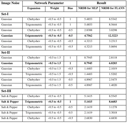
Table-1 Simulation Result

Image Noise

Network Parameter

Result

Expansion Weight Bias NRDB for MLP NRDB for FLANN

Set-I

Gaussian Chebyshev +0.5 to -0.5 1 5.4853 8.5342

Gaussian Trigonometric +0.5 to -0.5 1 5.4853 8.5644

Gaussian Chebyshev +0.5 to -0.5 -0.5 2.8388 3.0298

Gaussian Trigonometric +0.5 to -0.5 -0.5 4.7562 12.3223

Gaussian Chebyshev +0.5 to -0.5 +0.5 4.3213 3.2313

Gaussian Trigonometric +0.5 to -0.5 +0.5 4.3213 5.0694

Set-II

Gaussian Chebyshev +0.5 to 1.5 1 0.7945 2.8118

Gaussian Trigonometric +0.5 to 1.5 1 0.7945 6.0203

Gaussian Chebyshev +0.5 to 1.5 +0.5 1.4403 2.1019

Gaussian Trigonometric +0.5 to 1.5 +0.5 1.4403 1.5202

Gaussian Chebyshev +0.5 to 1.5 -0.5 4.8967 2.5475

Gaussian Trigonometric +0.5 to 1.5 -0.5 4.8967 1.4020

Set-III

Salt & Pepper Chebyshev +0.5 to -0.5 1 5.1415 8.5545

Salt & Pepper Trigonometric +0.5 to -0.5 1 5.1415 8.6683

Salt & Pepper Chebyshev +0.5 to -0.5 -0.5 2.1419 3.1278

Salt & Pepper Trigonometric +0.5 to -0.5 -0.5 2.1419 3.3018

Salt & Pepper Trigonometric +0.5 to -0.5 +0.5 2.6830 5.4700

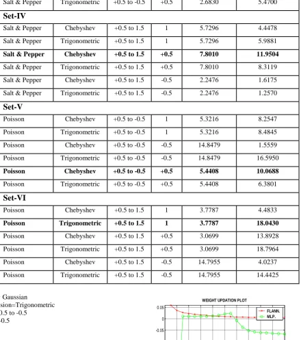
Set-IV

Salt & Pepper Chebyshev +0.5 to 1.5 1 5.7296 4.4478

Salt & Pepper Trigonometric +0.5 to 1.5 1 5.7296 5.9881

Salt & Pepper Chebyshev +0.5 to 1.5 +0.5 7.8010 11.9504

Salt & Pepper Trigonometric +0.5 to 1.5 +0.5 7.8010 8.3119

Salt & Pepper Chebyshev +0.5 to 1.5 -0.5 2.2476 1.6175

Salt & Pepper Trigonometric +0.5 to 1.5 -0.5 2.2476 1.2570

Set-V

Poisson Chebyshev +0.5 to -0.5 1 5.3216 8.2547

Poisson Trigonometric +0.5 to -0.5 1 5.3216 8.4845

Poisson Chebyshev +0.5 to -0.5 -0.5 14.8479 1.5559

Poisson Trigonometric +0.5 to -0.5 -0.5 14.8479 16.5950

Poisson Chebyshev +0.5 to -0.5 +0.5 5.4408 10.0688

Poisson Trigonometric +0.5 to -0.5 +0.5 5.4408 6.3801

Set-VI

Poisson Chebyshev +0.5 to 1.5 1 3.7787 4.4833

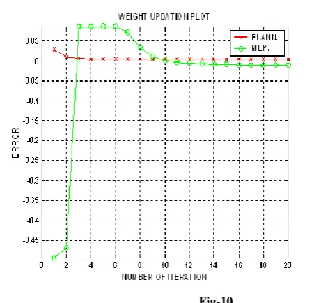
Poisson Trigonometric +0.5 to 1.5 1 3.7787 18.0430

Poisson Chebyshev +0.5 to 1.5 +0.5 3.0699 13.8928

Poisson Trigonometric +0.5 to 1.5 +0.5 3.0699 18.7964

Poisson Chebyshev +0.5 to 1.5 -0.5 14.7955 4.0237

Poisson Trigonometric +0.5 to 1.5 -0.5 14.7955 14.4425

Noise: Gaussian

Expansion=Trigonometric Wt=+0.5 to -0.5

Bias=-0.5

Fig-5

0 2 4 6 8 10 12 14 16 18 20

-0.45 -0.4 -0.35 -0.3 -0.25 -0.2 -0.15 -0.1 -0.05 0 0.05

NUMBER OF ITERATION

E

R

R

O

R

WEIGHT UPDATION PLOT

NRDB (FLANN) =12.3223 NRDB (MLP) =4.7562

Noise:Gaussian,

Expansion=Trigonometric Wt=+0.5 to 1.5

Bias=1

Fig-6

NRDB (FLANN) =6.0203 NRDB (MLP) = 0.7945

Noise: salt & pepper Expansion=Trigonometric Weight=+0.5 to -0.5 Bias=1

Fig-7

NRDB (FLANN) =8.6683 NRDB (MLP) =5.1415

Noise: Salt & pepper

Expansion=Chebyshev Weight=+0.5 to 1.5 Bias=+0.5

Fig-8

NRDB (FLANN) =11.9504 NRDB (MLP) =7.8010 Noise: - Poisson Expansion= Chebyshev Weight=+0.5 to -0.5 Bias=+0.5

NRDB (FLANN) =10.0688 NRDB (MLP) =5.4408

Noise: - Poisson

Expansion=Trigonometric Weight=+0.5 to 1.5 Bias=1

0 2 4 6 8 10 12 14 16 18 20

-0.04 -0.02 0 0.02 0.04 0.06 0.08

NUMBER OF ITERATION

E

R

R

O

R

WEIGHT UPDATION PLOT

FLANN. MLP.

0 2 4 6 8 10 12 14 16 18 20

-0.02 -0.01 0 0.01 0.02 0.03 0.04 0.05 0.06 0.07 0.08

NUMBER OF ITERATION

E

R

R

O

R

WEIGHT UPDATION PLOT

FLANN. MLP.

0 2 4 6 8 10 12 14 16 18 20

-6 -4 -2 0 2 4 6

x 10-3

NUMBER OF ITERATION

E

R

R

O

R

WEIGHT UPDATION PLOT

Fig-10

NRDB (FLANN) =18.0430 NRDB (MLP) =3.7877

Fig 11: Original Image

Fig 13: Filtered Image

Based on the analysis mentioned above we have de-noised the image corrupted by Gaussian noise by using FLANN network. First the noisy Cameraman image is passed through the single layer neural network shown in Fig-12 and the target was the original cameraman image Fig-11. After passing through FLANN network the image obtained result is shown in Fig-13. It is clear from result that image obtain is objectively better.

Irrespective of type of input noise whether Gaussian or Salt & pepper type it is found that NRDB for FLANN is always higher than MLP with variation of biases and weights for Trigonometric functional expansions.

4.

CONCLUSION

In this paper, we have proposed a novel adaptive image restoration method based on functional Link Artificial Neural Network to solve the problem of training convergence speed and computational complexity. The performance of FLANN has been studied and compared by means of simulations. Since the hidden layer is replaced by nonlinear functional expansions in this structure, the computational complexity is less thus; the learning rate is faster than that MLP. The prime advantage of this method is its reduced computational complexity with less number of biases and weights. The Simulation results indicate that performance of the proposed network is as good as that of MLP. The FLANN network may be used for on-line applications due to its less computational requirement and satisfactory performance. Image restoration using FLANN have an inherent limitation, of not guarantying universal approximation which has deterred interests among the researchers. Only a few application using M-FLANN are available in literature. Therefore, this has been a major motivating factor for using and exploiting M-FLANN in the field of image restoration.

5.

FUTURE WORK

Better result will come out if we will improve the performance of the network by using efficient algorithms for color images processing in internet & wireless applications.

6.

REFERENCES

[1] Rafal c. Gonzalez, Richard E. Woods, Digital Image Processing PHI, 2006.

[2] L.Yin, R.Yang, M.Gabbuj, and Y. Neuvo : “Weighted Median Filter: A Tutorial ”,IEEE Transaction, Circuits and

[3] D. R.K. Brownrigg: “The Weighted Median Filter” Communication. ACM, vol. 27, no. 8, pp. 807-918, August 1984.

[4] B. I. Justusson, “Median filtering: Statistical properties” Two-Dimensional Digital Signal Processing, T. S. Huang Ed., New York; Springer Verlag, 1981.

[5] T. Loupos, W. N. McDicken and P. L. Allan, “An adaptative weighted median filter for speckle suppression in medical ultrasonic images,” IEEE Transaction in Circuits Sysems., vol. 36, No. 1,pp.129-135, January 1989.

[6] Ghani. F, Khan. E, ”Missing lines recovery and impulse noise suppression using improved 2.-D median filters” IEEE Transaction on .Consumer Electronics, Vol. 45, No.2, pp. 356-360 May1999.

[7] Singh.K.M, Bora.P.K, Singh. S.B, "Rank-ordered mean filter for removal of impulse noise from images", IEEE International Conference, Industrial Technology, 2002, Vol. 2, pp.980-985 December 2002.

[8] A.Taguchi, M.Muneyasu and T.Hinamo T.Hinamoto “Median and Neural Network Hybrid (MNNH) Filters” IEICE (A) Vol. J-79-A, No.10, pp.1817-1825,Nov-1996. [9] R Grino. G. Cembrano and C.Torres. "Nonlinear system

identification using additive dynamic neural networks two on line approaches”. IEEE Transaction Circuits System I vol. 47 pp.150-165.Feb 2000.

[10] S. Chen .S. A. Billings and P.M Grant. "Recursive Hybrid Algorithm for nonlinear system identification using radial basis function networks”. International journal on Control. vol.55. no.5.pp.1051-1070, 1992.

[11] Q. Zhang and A. Benvenister. "Wavwlet networks “. IEEE Trans Neural Network vol 3 pp.889-898, Mar 1992.

[12] Y. H. Pao .Adaptive Pattern Recognition and neural networks. MA Addison-Wesley. 1989

[13] Patra, J. C, Pal R,N. Chatterji, B,N. Panda,G. “Identification of nonlinear dynamic systems using functional link artificial neural network”. IEEE Transactions, Systems, Man and Cybernetics, Part-B, Vol 29, pp.254-262, April-1999 [14] A. Namatame and N.Ueda. “Pattern classification with

Chebyshev neural networks”. International Journal on Neural networks, Vol. 3, pp.23-31, Mar 1992.

[15] Patra, J. C., Pal, R. N, “Functional link ANN based adaptive channel equalization of nonlinear channels with QAM signal”. IEEE International Conference, Systems, Man and Cybernetics, 1995, Vol-3, pp2081-2056, Oct-1995

[16] T. Chan, S. Esedoglu, F. Park, A. Yip “Recent Developments in Total Variation Image Restoration” UCLA Reports, 05-01.

[17] Singh Kh. Manglem, Bora Prabin K. “Adaptive Rank-ordered Mean Filter for Removal of Impulse Noise from Images”

[18] Patra J.C. , Kot A.C., “Nonlinear Dynamic System Identification Using Chebyshev Functional Link Artificial Neural Networks” IEEE Transactions on Systems, Man and Cybernetics, Part A: Systems and Humans - TSMCA , vol. 32, no. 4, pp. 505-511, 2002.