A complementary test for ADF test with an application to the exchange rates returns

Munich Personal RePEc Archive

A complementary test for ADF test with

an application to the exchange rates

returns

Liew, Venus Khim-Sen and Lau, Sie-Hoe and Ling, Siew-Eng

2005

A Complementary Test for ADF Test with An Application to the Exchange Rates Returns

Venus Khim-Sen Liew

Labuan School of International Business and Finance, Universiti Malaysia Sabah

Sie-Hoe Lau

Faculty of Information Technology and Quantitastive Science, Universiti Teknologi MARA, Sarawak Campus

Siew-Eng Ling

Faculty of Information Technology and Quantitastive Science, Universiti Teknologi MARA, Sarawak Campus

Abstract

A Complementary Test for ADF Test with An Application to the Exchange Rates Returns

1. Introduction

A basic requirement for time series modelling is that the series under study must be weakly stationary, i.e. it has constant mean and covariance. Numerous stationary tests have been developed in the past to test for stationarity and the popularly applied tests include the augmented Dickey-Fuller (ADF) test (Fuller 1976, Dickey and Fuller 1979), Phillips-Perron (PP) test (Phillips 1987, Phillips and Perron 1988) and Kwiatkowski-Phillips-Schmidt-Shin (KPSS) test (Kwiatkowski et al. 1992). Lately, Ahamada (2004)

demonstrates via a simulation exercise that KPSS test fails to detect a form of nonstationarity due to a shift in the unconditional variance. They pointed out that the non-rejection of the null hypothesis of no unit root in the KPSS test does not neccesarily imply the stationarity of the data, as there is a possibility that the data may exhibit heterogeneous unconditional variance. The author further proposed a complementary test to complete the KPSS testing procedure and the complementary test was shown to be useful detecting the nonstationary covariance of the daily returns of US dollar/Euro exchange rate, in which the KPSS test has failed to do so.

complementary test as proposed in Ahamada (2004) in correctly identifying simulated series of nonstationary covariance is also scrutinized in this simulation study.

To preview our findings, the current study discovers that the ADF test has identified the simulated nonstationary covariance as stationary series with a unit probability. Similar finding is observed in the DF test, which is included in this simulation study for comparison purpose. On the other hand, using the complementary test as proposed in

Ahamada (2004), nonstationary covariance has been correctly identified in almost all cases. Hence, this study proposes the use of this complementary test in the case of ADF test to detect nonstationary covariance if ADF test suggests no unit root in the series of interest. In this regards, the current study simulates and reports the critical values of this complementary test. In addition, this study applies the same complementary test in the case of ADF (hereafter referred as complementary ADF test) to the returns of few US dollar based exchange rate series of some developed countries to illustrate the usefulness of this complementary ADF test.

2. The Complementary ADF Test

Ahamada (2004) wisely tailored the cumulative sum of square (CSS) procedure in Inclán and Tiao (1994) to formulate a complementary test for the KPSS testing procedure (hereafter, complementary KPSS test). This useful test is easily applied and interested readers may refer to Ahamada (2004)1. In the vein of Ahamada (2004), this study extends the application of the same CSS procedure in the case of ADF, yielding to the so-called complementary ADF test2.

Consider the following time series {y_t}, which is stationary around the level r₀:

t

y = r₀+ε_t, t=1,...,T, (1)

where ε_t is independent and identically distributed (i.i.d.) with a zero mean and constant variance, denoted ε_t ~ i.i.d.(0, σ_ε2).

The stationarity of {y_t} may be tested by the augmented Dickey-Fuller (ADF) test3:

1

Available at http://www.economicsbulletin.com/2004/volume3/EB-03C10010A.pdf.

2

For compatibility, the current study follows closely the definitions and notations in Ahamada (2004).

3

ADF is the improved version of Dickey-Fuller (DF) test of the framework∆y_t =∂y_t−1+ω_t, where ω_t

~ i.i.d. (0, σ_ω2). Here, the null hypothesis of ∂=1 (unit root) is tested against the alternative hypothesis of

t

y

∆ = _t

p

i

i t i

t y

y

∑

= −

− + ∆ +

∂

1

1 , (2)

where η_t ~ i.i.d.(0, σ_η2), p is the autoregressive lag length large enough to eliminate possible serial correlation in η_t and ∂ is the coefficient of interest. Conventionally, if ∂ = 0, the series contains a unit root implying nonstationary, whereas if ∂ < 0, there is no unit root implying stationarity. In the ADF test, the null hypothesis of unit root, i.e.

ADF

H₀ : ∂ = 0 is tested against the alternative hypothesis of no unit root, i.e. H_AADF: ∂ < 0 using the t test of individual significance.

It is obvious that under the generating mechanism in (1) with ε_t ~ i.i.d.(0, σ_ε2), ∂ in (2) equals 0, thereby conventionally one may conclude that {y_t} is stationary. The concern of this study is whether or not the ADF test is robust against heterogeneous variance process i.e. E(ε_t2) = σ ≠_t2 σ_ε2. In this regard, a simulation study has been conducted and we will see shortly that ADF test had identified nonstationary covariance series as stationary process4. A complementary test for ADF test is therefore needed to differentiate completely stationary process (mean and covariance stationary) from mean stationary but covariance nonstationary process. As in Ahamada (2004), the current study utilises the supremum T/2|D_K | statistic proposed in Inclán and Tiao (1994), defined as5:

4

Although striking, the results come as no surprise as Ahamada (2004) has already shown similar failure of the most powerful unit root test.

5

τ = max /2| | ,...,

1 T K

k= T D (3)

where T k C C D T k

k = − , Ck= , 1,..., . 1 2 T k e k t t =

∑

e in turn is the ordinary least squares (OLS)

residuals from regressing {y_t} on a constant as in (1). Under the null hypothesis of e_t is independent and identically distributed with zero mean and homogeous variance, i.e.

C

H₀ : e_t ~ i.i.d. (0, σ_e2), Ahamada (2004) showed that the limiting distribution of τ is given by one of the sup{W_t0}, where W_t0 is a standard Brownian Bridge. It is noted here that the above assumption is also valid and therefore the distribution of sup{W_t0} given by Billingsley (1968) is applicable in the current case6:

{

}

2 1 0 ) 1 ( 2 1 | | sup

Pr k b

k

k

t b e

W − ∞ =

∑

≤ , b > 0 (4)

where }Pr{A denotes the probability of event A occurs and b is the critical value. Based on simulation exercises done by Inclán and Tiao (1994), the asymptotic 10%, 5% and 1% critical values for τ are corresponding 1.224, 1.358 and 1.6287.

6

See proof of Proposition 1 in Ahamada (2004) and proof of Theorem 1 in Inclán and Tiao (1994).

7

With the availability of this complementary ADF test, we may now conduct a complete ADF test by carrying out the following two-step procedure8: First, apply the ADF test. If the null hypothesis is not rejected, then we may conclude that the data is nonstationary, i.e. it contains a unit root. If the null hypothesis is rejected, there is no unit root but a shift in the variance is possible. For this case, we suggest to apply the complementary ADF test. If the τ statistic fails to reject the null hypothesis, then we have enough statistical evidence to conclude that there is a complete covariance stationarity. Otherwise, the data have variance shift and the process is not covariance stationary although there is no unit root.

3. Simulation Procedures and Results

Consider the following data-generating processes (DGP) specified in Ahamada (2004):

0 H

DGP : x_t =0.01+ε_t, (5)

where ε_t~N(0,1) for t = 1, …, 200; and

' 01 . 0

: _{t t}

H y

DGP

A = +ε , (6)

8

where ε_t'~N(0,1) for t = 1, …, 100 and ε_t'~N(0,1.5) for t = 101, …, 200.

Note that the series {x_t} is stationary around the level 0.01 but {y_t} is nonstationary as the variance varies. The estimated rejection rate of the null hypothesis of nonstationary at 1%, 5% and 10% level for both series for 1000 replications of each DGP is given in Table 1.

TABLE 1. Rejection Rate of the Null Hypothesis of Nonstationary

Series DF Test ADF Testa Complementary Test

10 5% 1% 10% 5% 1% 10 5% 1%

{x_t} 1.000 1.000 1.000 1.000 1.000 1.000 0.116 0.051 0.012 {y_t} 1.000 1.000 1.000 1.000 1.000 1.000 0.883 0.957 0.989

Note: a Results reported are for p= 4. Similar results (not shown) are obtained with other specifications of

p.

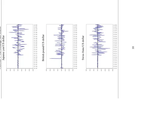
4. Illustrations of Complementary ADF Test

10

finding on the daily returns of US dollar/Euro

exchange rate by the com

p

lem

entary KPSS

test.

FIGURE 1. The exchange rate returns

Japanse yen/US dollar

-0 .0 8 -0 .0 6 -0 .0 4 -0 .0 2 0.00 0.02 0.04 0.06 Q1 1957 Q1 1959 Q1 1961 Q1 1963 Q1 1965 Q1 1967 Q1 1969 Q1 1971 Q1 1973 Q1 1975 Q1 1977 Q1 1979 Q1 1981 Q1 1983 Q1 1985 Q1 1987 Q1 1989 Q1 1991 Q1 1993 Q1 1995 Q1 1997 Q1 1999 Q1 2001 Q1 2003

British pound/US dollar

-0 .0 6 -0 .0 4 -0 .0 2 0.00 0.02 0.04 0.06 0.08 Q1 1957 Q1 1959 Q1 1961 Q1 1963 Q1 1965 Q1 1967 Q1 1969 Q1 1971 Q1 1973 Q1 1975 Q1 1977 Q1 1979 Q1 1981 Q1 1983 Q1 1985 Q1 1987 Q1 1989 Q1 1991 Q1 1993 Q1 1995 Q1 1997 Q1 1999 Q1 2001 Q1 2003

Swiss franc/US dollar

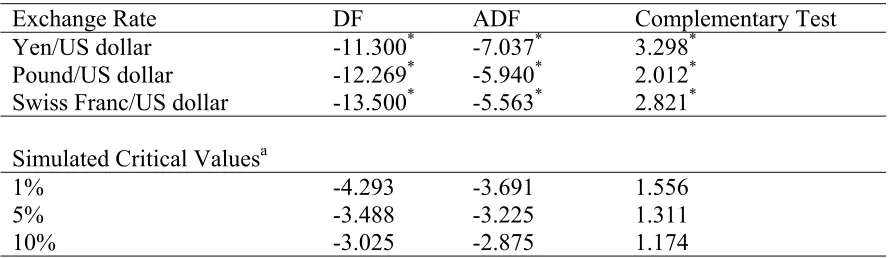
TABLE 2. DF, ADF and complementary tests results with simulated critical values

Exchange Rate DF ADF Complementary Test

Yen/US dollar -11.300* -7.037* 3.298* Pound/US dollar -12.269* -5.940* 2.012* Swiss Franc/US dollar -13.500* -5.563* 2.821* Simulated Critical Valuesa

1% -4.293 -3.691 1.556

5% -3.488 -3.225 1.311

10% -3.025 -2.875 1.174

Note: a Estimated from 1000 replications of 188 independent N(0,1) observations. Asterisk (*) denotes significant at 1% level.

5. Conclusion

This study demonstrates through a simulation study that the most commonly applied ADF test failed to detect covariance nonstationary series. This finding is not surprising as

results, it is concluded that these exchange rate returns are covariance nonstationary although there is no unit root.

References

Ahamada, I. (2004) “A complementary test for the KPSS test with an application to the US dollar/Euro exchange rate” Economic Bulletin3(4), 1 – 5.

Billingsley, P. (1968) Convergence of Probability Measures, John-Wiley: New York. Dickey, D. (1976) Introduction to Statistical Time Series, Wiley: New York.

Dickey, D. and W. A. Fuller (1979) “Distribution of the Estimators for time series

regressios with a unit root” Journal of the American Statistical Association74, 427 – 431. Inclán, C. and G.C. Tiao (1994) “Use of cumulative sums of squares for retrospective detection of changes of variance” Journal of American Statistical Association 89, 913 – 923.

Phillpis, P.C.B. (1987) “Time series regression with a unit root” Econometrica55, 277 – 301.

Phillips, P. C. B. and P. Perron (1988) “Testing for a unit root in time series regressions”

Biometrika 65, 335 – 346.

APPENDIX 1

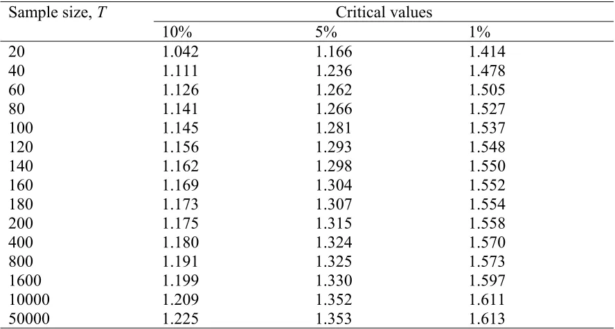
TABLE 3. Critical values of τ statistic for various sample size, T. Critical values

Sample size, T

10% 5% 1%

20 1.042 1.166 1.414

40 1.111 1.236 1.478

60 1.126 1.262 1.505

80 1.141 1.266 1.527

100 1.145 1.281 1.537 120 1.156 1.293 1.548 140 1.162 1.298 1.550 160 1.169 1.304 1.552 180 1.173 1.307 1.554

200 1.175 1.315 1.558

400 1.180 1.324 1.570

800 1.191 1.325 1.573

1600 1.199 1.330 1.597

10000 1.209 1.352 1.611 50000 1.225 1.353 1.613

Note: Estimated from 10000 series that are replicated from independent random errors with N(0,1) distribution. Each series contains T usable observations.

TABLE 4. Critical values of τ statistic for various residuals variance,σ_ε2. Critical values

2

ε σ

10% 5% 1%

0.1 1.197 1.336 1.597

1 1.205 1.352 1.612

10 1.211 1.355 1.616