Munich Personal RePEc Archive
The Role of Foreign Aid and the Foreign
Exchange Constraint in Growth: Some
Extensions
Goyal, Ashima
Indira Gandhi Institute of Development Research
1993
Online at
https://mpra.ub.uni-muenchen.de/73179/
1
Preprint from Journal of Foreign Exchange and International Finance 8(1), pp. 30-43. 1993
The Role of Foreign Aid and the Foreign Exchange Constraint in Growth: Some
Extensions∗∗∗∗
Ashima Goyal
Indira Gandhi Institute of Development Research Gen. Vaidya Marg, Santosh Nagar,
Goregaon (E), Mumbai-400 065 ashima @ igidr.ac.in
Tel.: +91-22-28416512 Fax: +91-22-28402752
http://www.igidr.ac.in/~ashima
Abstract
An analytical framework that draws both upon the two-gap models and work on non-market clearing short-run constrained equilibria, and its application to long-run growth, is applied to find out when the contribution of foreign resources to growth is maximum. A theoretically consistent treatment of foreign inflows, starting from consumer and firm decisions, shows that foreign inflows need not have a negative coefficient in a behavioural savings function. A model with a saving function, an investment function and an import constraint generates a demand constrained short-run equilibrium in addition to savings and trade and capacity constrained equilibria. Considerations of dynamics and long-run persistence of constraints and equilibria, show foreign inflows make the maximum contribution, when the resource and trade constraints are binding, since rise in output and domestic savings results in the
maximum increase in investment. Simulations show such a virtuous growth path was reversed in the sixties and seventies in India. A sudden fall in inflows reduced the slope and intercept of the investment function and the economy shifted to a stagflationary trajectory.
Keywords: Two-gap models; Constrained equilibira; Foreign exchange constraint; Dynamics; Growth paths.
JEL classification code: F31, F35, F43, O11
∗
2
I. Introduction
The objective is to take a fresh look at the contribution of foreign resources to development. Do foreign resources lead to an increase in savings, investment and growth? Under what conditions are their contribution maximized? An analytical framework that draws both upon the two-gap models and work on non-market clearing short-run constrained equilibria, and its application to long-run growth (see Malinvaud 1980), is developed and applied to analyze the impact of aid flows on the Indian growth experience.
The conceptual issues are developed in the next section. Then some suggestions are made for ensuring a theoretically consistent treatment of foreign inflows, starting from consumer and firm decisions. In section 4, a model that generates demand, capacity or trade constrained short-run equilibria is developed. The different constrained regimes obtained are studied and the productivity of aid under each regime as well as the relationship between aid and
domestic savings are examined. Some extensions are carried out by incorporating dynamic considerations in analyzing the effect of foreign inflows on investment. Finally, simulations are carried out in a dynamic model of the Indian economy.
II. Substitution and Constraints
Initially two gap models were used to analyze the effects of savings and foreign exchange constraints on output and growth. Recently fiscal and inflationary constraints have been added to the list. The models are commonly specified in terms of macroeconomic variables, and where the adjusting variables are less than the number of constraints, imply that some resource remains underutilized, with the binding constraint restricting growth. Foreign
inflows, (F) contribute by relaxing a binding constraint and allowing fuller utilization of other resources. In the literature different constraints are shown to bind at different levels of F.
Figure 1, following Weisskopf (1972) shows three possible equilibrium (A, B, C) combinations of investment, I and income Y, depending on which pair of simple linear import (E+F), resource (S+F) or capacity, Y, constraints bind. The import constraint shifts out comparatively more than the savings constraint as foreign aid rises from F1 to F2.
3
short-run constraint1 because of import substitution and export promotion possibilities, especially in a country with a developed industrial base. In section 5 we see that a strict linear import constraint did not hold for the Indian economy. Further, an equilibrium such as B is unlikely to occur.
1
4
Consumers will not save less than they desire. Market adjustments, combined with
5
There has been recent work on the long run persistence of demand constrained equilibria with excess capacity. Goyal (1989) shows how this is consistent with profit maximizing behaviour of price setting firms. It is correct to assume that all savings will be invested, only in plan models such as the original two-gap models, or else in models with perfect foresight and futures markets and zero installation costs. Otherwise an independent investment function is required. The fiscal constraint in three gap models is often developed from the trade-off between public and private investment and forced savings through inflation. In the model developed in section 4, investment is linked to output through separate private and public sector investment functions. Public sector investment can be ‘crowded out’ in periods of high inflation. The model is used to examine the effect of an import constraint on the evolution of short-run demand constrained equilibria.
It follows that useful distinctions to be made are: (a) between constraints that are primarily technological and those that are behavioural. Examples of the former are the import and the capacity constraints. They will shift in the long-run while behavioural constraints such as savings and investment may persist; (b) constraints that are likely to persist and (c) the relationship between constraints.
In the model developed below, a simple linear savings function with a fixed propensity to save, out of non-agricultural profit income, is used. Life cycle utility maximization with a bequest motive, only for the rich and liquidity constraints for the poor, can generate a savings function, with a very low or zero propensity to save out of wages and a high propensity to save out of profit income. The rate of interest will affect savings only if the intertemporal elasticity of substitution of consumption is high, although the allocative effects of the interest rate are important. The parameters of the savings function can change in a Lucasian fashion with shifts in the expected growth paths. The life cycle hypothesis will also imply differing saving propensities out of domestic and foreign resources. In the literature following the two gap models, arguments were advanced for expecting a negative coefficient of F in the savings function2. It is shown in the following section that this was derived merely from the ex-post savings, investment tautology, ignoring the fact that ex-ante investment and consumption or savings decisions are independent. Early empirical results showed a negative coefficient of F
2
6
in a simple linear savings function estimated by ordinary least squares3. However, these studies had a number of data and estimation problems and newer studies have reversed the results4.
Finally, the model used implies an empirically based judgement, of which constraints and adjustment dynamics have been important in the Indian economy in the past thirty years. Over much of the period, the short-run equilibrium was demand constrained. Even though a strict linear import constraint did not hold, shocks in F led to changes in parameters affecting demand. This provides a possible explanation of high and low medium-run growth.
III. Aid and Savings
The theoretical argument in justification of a negative coefficient for foreign aid in a behavioural savings function, may be represented algebraically as follows, given:
An investment function: I = i1 Y + i2F (1)
The ex-post identity: I SD + F (2)
We assume that F is the trade deficit financed by foreign inflows net of changes in foreign reserves. Substituting equation (1) in equation (2) and solving in terms of SD yields:
= + − 1 3
If i2 < 1, the coefficient of F in Equation (3) will be negative.
Savings in equation (3) are not behavioural and are obtained from the investment function given the ex-post equality of savings and investment. The household’s decision to distribute its income between consumption and savings is different from the firm’s decision to invest. The two must be kept distinct.
If investment is to be made a function of total resources, so that only a part of F is invested, it follows that a part of F will be consumed. So consumption also becomes a function of total resources.
3
See for example Griffin and Enos (1970), Weisskopf (1972), Grinols and Bhagwati (1976).
4
7
The consumption function would then become,
= + , 0 < < 1, 0 ≤ < 1 4
Substituting the consumption and investment functions in the macroeconomic identity Y + F C + I, we obtain:
1 − + 1 − ≡ + 5
Or,
+ ≡ + 6
So that behavioural savings are also a function of total resources, with different propensities to save out of Y and F.
The accounting convention (equation (2) above) says that gross domestic savings can be measured by subtracting foreign inflows from investment, even if a part of F is consumed, on the grounds that F has to be repaid and therefore leads to a drain on future savings. However, since F is measured in net terms, current repayments are accounted for. Future repayments would influence the savings decision from foreign resources. The convention should merely be taken to state that either domestic or foreign resources must finance investment in the current period. If the traditional procedure is followed, then:
Gross domestic savings = − ≡ + − 7
It is artificial to keep F on the right hand side, once F enters the behavioural consumption and investment functions. We can write equation (6) as,
+ * ≡ + 8
Where SD = s1Y is savings out of domestic income and SF = s2F is savings out of foreign
inflows.
The ex-post identity equation (2) should then be replaced by equation (8).
However, it is incorrect to treat domestic resources (Y) and foreign resources (F) as
equivalent. This was the suggestion Haavelmo originally made that started the literature on aid and savings. The scarcity of foreign inflows and repayment considerations impute a higher opportunity cost to foreign inflows consumed. This suggests that the s2 and i2
coefficients are likely to be much higher than the s1 and i1 coefficients. From a life cycle
8
decision only if the productivity of F exceeds the interest cost. Short-run liquidity constraints, or restructuring of consumption profiles over time, may explain current F entering the
consumption decision.
Equation (6) has some interesting implications. Adding an autonomous investment term I^, it becomes:
+ ≡ + + +∧ 9
If we assume that F is either consumed or invested, so that,
+ = 10
Or,
+ = 1
Then,
= 1 −
Now
= 1 −
And therefore,
= 11
So that equation (9) reduces to,
= +∧+ 12
Or
= +−∧ 13
An implication of the above equation is that, an equality between ex-post domestic savings and investment is brought about by multiplier changes in domestic income. Foreign inflows drop out of the equation and have no effect on short run income. In any case foreign inflows are exogenous they cannot vary to equate saving and investment gaps.
If all the foreign inflows are neither consumed nor invested so that s2 F > i2 F, we have5,
= − − + +∧ 14
Or domestic income would have to decrease until domestic saving decreases sufficiently to compensate for the excess of saving over investment out of foreign inflows.
5
Where foreign inflows are not net of changes in reserves, R, we have M - E = F - ∆R, then ∆R, or the change
in reserves, is added to the numerator of the RHS of equation (14). If all F is spent we would have (i2 – s2) F =
∆R, so that again, the numerator of (14) would be only I^
9
If i2F is invested, 0 < i2 < 1 and no F is consumed so that s2 = 1,
= − 1− + +∧ 15
Implying that the difference 1- SD = F is maintained by a decrease in income leading to a fall
in SD, as investment increases only by i2F.
It is only in this case that domestic savings (but not behavioural savings) decrease by an increase in F. This may have happened in India for a few years in the late seventies when a sudden rise in remittances contributed to a rise in the savings-output ratio. Domestic investment and output, increased only after a lag so that F was negative for three years and foreign exchange reserves accumulated.
IV. Constrained Equilibria
Short-Run Equilibria with Constraints: To examine different possible short-run equilibria and the productivity of F in each, a simple aggregative model is built that allows for separate savings and investment constraints on output, as well as trade and capacity constraints. Foreign inflows affect savings and investment according to the arguments made in section 3. The investment function is obtained by aggregating over private and public sector
investment. Private sector investment is derived by the maximization of expected returns from the construction of new capacity, by a representative firm (see Malinvaud 1980). The arguments of the function are (i) demand and profitability, proxied by the gap between output, Y and capacity, 1; (ii) profit income, τY, where τ is the firm’s mark-up. Public sector
investment is derived from the public sector budget constraint. ‘Reverse crowding out’ occurs with public sector investment tending to fall in periods of high price increase, so that we may postulate, that it is an increasing function of domestic and foreign resources (see Goyal 1989). I^ is the exogenous part of investment, * stands for desired quantities. Sectoral
interactions are abstracted from, or subsumed in the exogenous terms. For example, Y refers to manufacturing output and it is assumed that investment comprises only of manufacturing sector products, while the exogenous part of the savings function, S^ , includes agricultural and government savings.
10
exchange constraint states that actual imports M, which are determined by exogenously given foreign inflows F and exports E, cannot be less than required imports, M*. The latter are a linear function of output and investment, with the import coefficient for investment, f2,
exceeding that for output. The constant f0 allows the marginal import propensity to differ
from average.
+ = 16
= 2 − 3 17
∗ = ∧+ 5 + 6 18
2 ≥ 2∗ = 89+ 8 + 8 + 19
+ ≤ +∗ = +∧+ 6 − : + 6 + 6;5 20
Substituting equation (16) in (18), and equation (17) in (19) we obtain the four constraints restricting output and investment. These are:
The resource constraint, R:
+ − 5 = ∧+ 6 21
The trade constraint, T:
+ + 8 8< ≤ − 89 + 8 + 3 8< 22
The investment function, I:
+ − 6 + 6;5 ≤ +∧− 6 : + 6 23
The capacity constraint::
≤ : 24
There are four equations and two variables, I and Y, thereby providing us with two degrees of freedom. These can be filled up, by putting equalities, for any two of the constraints.
According to the argument in section 2, behavioural savings will always be realized, so that the combination of the resource constraint, with anyone of the others, will generate the possible short-run equilibria. Figures 2 and 4 demonstrate diagrammatically the constraints and different possible equilibria. In Figure 2, the possible equilibria are A and D. When equilibrium A holds, the constraint set is ORAT, with the resource and trade constraint binding. Investment is less than the desired value and there is excess capacity. This
corresponds to the A equilibrium of Figure 1. An increase in F would cause the constraint set to shift to OR′DEBY1, with outward shifts in the resource, investment and trade constraints.
11
long as a2 < (1/f2), a condition likely to hold true for a large, industrialized developing
country with a low import coefficient for investment.
The new equilibrium is at D, the demand constrained equilibrium where investment and savings are at their desired levels, there is excess capacity and the trade constraint does not hold. Investment and output are both higher than at A. As discussed earlier, B is not feasible as an equilibrium in a market economy. Similarly at E, excess savings would cause
investment and income to fall to D.
In Figure 3, with the constraint set ORCY1, the resource and capacity constraint would hold, leading to an equilibrium at C.
Here also, an increase in F, by shifting upwards the resource constraint, would increase investment and consequently capacity and output in the next period.
Figure 4 shows the case of short-run instability. Output and investment would either
decrease, or increase explosively until restrained by the trade constraint at F or the capacity constraint at G.
Some comparative static results regarding the effects of an increase in exogenous foreign inflows on output and investment in each of the three possible equilibria A, D and C6 can be obtained by solving each combination of two constraints for output and investment.
(i) Equilibrium A with M = M*, S = S*, Y < Y1, I< I*
>
> = 8 + 8 5 > 01 − 8 6 25
6
There is a remote possibility of other unlikely equilibria occurring, if three constraints were to hold at the same time. The model then becomes overdetermined so that such equilibria would be possible only under special conditions on the exogenous variables. The conditions are, for equilibria with:
(i) S = S*, I = I*, M = M*, Y < :
5 − 6;5 − 6 @ 1 − 6 8 : + 3: − 89A − 8 + 8 5 +∧ + 56 8 + 6 8 : = − ∧@8 + 8 6 + 6 A
(ii) Y = :, I = I*, S = S*, M > M*
: − 6;5 = +∧− ∧
(iii) Y = :, S = S*, M = M*, I < I*
12
>+
> = 5 1 − 8 68 + 8 5 + 6 > 0 26
(ii) Equilibrium D with S = S*, I = I*,M > M*, Y < Y1
>
> = 0 27
>+
> = 6 > 0 28
Only in the case where savings out of foreign aid exceed investment out of it (see equation (14)) would income fall with an increase in foreign inflows.
(iii) Equilibrium C with Y = Y1, S = S*, M > M*, I< I*
>
> = 0 29
>+
> = 6 > 0 30
Thus, foreign inflows make the maximum contribution, in this model, in case A where the resource and trade constraints are binding. In all the cases, investment increases by the amount of foreign inflows invested (a2F), but only in case A does the relaxation of the trade
constraint allow output and domestic savings to increase. And therefore the increase in investment in this case exceeds a2F. The next question to be asked is if these results continue
to hold, when dynamics of movements from and approach to, equilibria are introduced.
If investment, particularly public sector investment (as was expected in the two-gap models), responds to foreign resources available, an equilibrium such as D, where excess foreign resources are available, should not persist. We would expect either that the investment function would shift upwards over time, or that the investment propensities would increase.
Dynamic Adjustments: Considering an example of the former case, first, we examine the dynamic adjustments when investment increases, with a lag, in response to, an excess of foreign inflows available relative to those used, in a short-run equilibrium such as D.
The resource constraint and the investment function are now, respectively, given by:
+B= ∧+ 5 B+ 6 B 31
13
where the subscript t stands for time. The solution value of investment is,
+B = 5 − 6− 56C8
;5 − 6 +BD + E 33
where
E = 5 − 65
;5 − 6 +
∧+ 6 B+ 6C BD + 6C3BD − 6C89− 6 :B− 8 6C BD − 6 ∧
− 6;5 ∧ 34
The general solution for this linear first-order non-homogenous difference equation is:
+B = F 5 − 6− 56C8 ;5 − 6 G
B
+ E+ + F
56C8
5 − 6;5 − 6 G B
+ + F 56C8
5 − 6;5 − 6 G
35
+B= F 5 − 6− 56C8 ;5 − 6 G
B
+ E 5 − 65 − 6;− 6
;5 − 6 + 56C8 36
The value of the root, though very small, is negative and will cause damped oscillations. It arises from the negative effect of the 2B∗ terms on It. However, the change in It will be
dominated by the particular solution which is positive. Therefore, in this model, It will
increase as long as B + 3B > 2B∗. The investment function in case D will shift upwards.
If multiplier instability holds, so that 5 − 6;5 − 6 < 0, the root will also be positive.
Where public investment is primarily constrained by resources and private investment by expected profitability, a relaxation of the foreign exchange constraint may result in investment propensities exceeding savings propensities. This can be proved in a model (Goyal 1989), with rational expectations over dynamic adjustment paths. Equation (20) subsumes a public sector investment function which depends positively on household savings. In the Indian economy household savings, remittances from abroad and foreign exchange reserves rose in the late seventies. This led to a policy of deliberate budget deficits (financed partly by increased borrowing from households), for drawing down the reserves (see Shetty and Menon 1980). Such behaviour could imply an unstable short-run multiplier as government propensity to invest out of household savings increased with F, leading to
14
In Goyal (1989) it is shown that in a model where the short-run Keynesian multiplier can become unstable, restrictions on price setting behaviour, obtained from profit maximization by a representative firm, provide an explanation for both limited flexibility in real prices and the behaviour of historical aggregate output and price. In empirical simulations with the model, historical price and output series for the Indian economy were reproduced along smooth dynamic trajectories approaching different equilibria.
Along high growth trajectories savings increase to match investment partly through rising incomes and partly as high returns attract savings from agriculture and the parallel economy. The constraint R may shift, reducing some crowding out of desired investment as occurs at F (Figure 4).
Bacha (1990) has an opposite result where a fiscal constraint may crowd out investment, even with excess F, in a country with a low f2. In his model, savings going to the public sector can
be increased only by seigniorage. In the Indian economy, in the eighties, increased savings were allocated to the public sector by borrowing. Some results in Goyal (1991) indicate that savings and their allocation is a rising function of growth and returns, respectively. So that low cost policies can be designed to increase the share of public sector savings and maintain investment. It is possible that a virtuous growth path without seigniorage may be sustained at a rate where rising investment continually shifts back the capacity, savings and trade
constraints (through falling f2 and capital-output ratios). Another point to note is, that a
suggestion sometimes made for utilization of excess F, increasing f2 or reducing import
controls, would reduce the above expansionary effects of F on I and Y.
Simulations with the Indian economy suggest that the reverse of such a virtuous growth path occurred in the sixties and seventies, coinciding with a sudden fall in F. The slope and intercept of the investment function declined and the economy shifted to a stagflationary trajectory. Something similar may also occur now, in the early nineties. This argument underlines the importance of large aid or foreign direct investment inflows for the continued growth of the Indian economy.
15
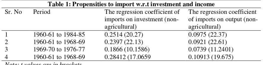
[image:16.595.64.508.155.265.2]Was the foreign exchange constraint important in explaining features of Indian economic growth? Given India's large industrial base and the government’s policies of import restriction, it is unlikely that the strict linear import constraint held.
Table 1: Propensities to import w.r.t investment and income
Sr. No Period The regression coefficient of
imports on investment (non-agricultural)
The regression coefficient of imports on output (non-agricultural)
1 1960-61 to 1984-85 0.2514 (20.27) 0.0975 (22.37)
2 1960-61 to 1968-69 0.2397 (22.13) 0.0921 (22.61)
3 1969-70 to 1976-77 0.1866 (10.1586) 0.0739 (11.2401)
4 1960-61 to 1968-69 0.28412 (17.0659 0.10913 (19.675)
Note: t values are in brackets
Attempts were made to estimate a required imports function of the form of equation (19). To take account of changes in coefficients, regressions were run for the whole period, as well as for the sub-periods 1960-61 to 1968-69, 1969-70 to 1976-77, and 1977-78 to 1984-85. A number of alternative variants were tested, but the results were found to be satisfactory only when non-agricultural output and investment were regressed separately on the historical series for non-agricultural imports M(H)7, without an intercept term. Using nominal variables, their first differences, or moving averages, did not improve the regressions. The coefficients for M = bI and M = cY are given in Table 1. The t values are in brackets. It may be that the conventional form of the import constraint is inadequate as substitution occurs, or that a simultaneous equation bias did not allow its accurate estimation by OLS.
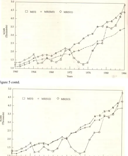
Empirical simulations with a dynamic model for the Indian economy (see Goyal 1989 and also the appendix for a brief outline) show that the values of output and investment generated by a variety of linear import constraints in years when required imports were greater than
M H (or historical F + E), are too low compared to historical values. This also suggests that in years when there was a fall in M H , forced substitution took place, so that the linear import constraint did not hold. These simulations also show required imports MR, exceeding
M H in the years 1965-66 to 1968-69 and 1973-74 to 1978-79. Only one of these
simulations SM5, is reported in Figure 58. Of course, the negative NCI during 1975-76 to
7
Historical import series M(H) for the non-agricultural sector were obtained by adding net invisibles to the historical import series and then subtracting imports of food and deflating the resulting estimates by the price index of imports. M H series were obtained by adding exports (plus positive net invisibles) to net capital inflow (NCI) and deflating the resulting estimates by the price index of imports.
8
16
1978-79 contributed to M being low and therefore these years cannot be regarded as being import constrained.
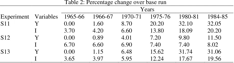
A hypothetical experiment was designed to capture the effect on investment if there had been no decrease in M in the late sixties and early seventies and as argued above, a decrease in the availability of resources would negatively affect investment propensities. Therefore, in simulation S11, the government or private propensity to invest was increased by 30 per cent after 1964-65 as compared to the base run, or the simulation that closely reproduced the historical series. In S12, instead of the increase in investment propensity, an equivalent increase in autonomous government investment of Rs. 400 crores, is added. This is also equivalent to the difference in M(H) between 1964-1965 and 1972-73, or to the decrease in net capital inflow that took place during this period. In S13, autonomous savings are increased by Rs. 400 crores and investment propensities are increased by 30 per cent after 1964-65.
[image:17.595.71.530.494.618.2]In all the three cases the resultant required imports9 series do not show the decrease that occurred in the M(H) series and reach the M(H) peaks of Rs. 2177 crores in 1971-72 and Rs. 125 crores in 1983-84 almost exactly (see Figure 5). Table 2 gives the percentages by which investment and income exceed the historical level in selected years.
Table 2: Percentage change over base run Years
Experiment Variables 1965-66 1966-67 1970-71 1975-76 1980-81 1984-85 S11 Y 0.00 1.60 8.70 20.20 32.10 32.05
I 3.70 4.20 6.60 13.80 18.09 20.20 S12 Y 0.00 0.89 4.01 7.20 9.80 11.50 I 6.70 6.60 6.90 7.40 7.40 8.02 S13 Y 0.00 1.15 6.48 15.62 31.74 31.06
I 3.65 3.97 5.95 12.24 17.67 19.56
S13 may be taken as an experiment that demonstrates that, ceteris paribus, if there had not been the historical fall in M in the late sixties and early seventies and a consequent decline in investment propensities, Y in 1984-85 would have been as much as 32 per cent higher than its historical level.
9
17
Figure 5
Figure 5 contd.
VI. Conclusion
18
coefficient for foreign inflows in a behavioural savings function was unsound. In section 4, it was seen that a model incorporating a theoretically consistent saving function, an
independent investment function and an import constraint generates a demand constrained short-run equilibrium in addition to savings and trade and capacity constrained equilibria. The contribution of foreign inflows to output and investment was obtained under each of the possible constrained short-run regimes. Considerations of dynamics and long-run equilibria, briefly examined, suggest that the contributions of foreign inflows could be quite large. It seems that in the Indian economy the foreign resources constraint may form part of the
explanation for the persistence of an excess capacity demand constrained equilibria. Although a strict linear import constraint may not have held, because of substitution possibilities, so that foreign exchange may not have been a serious constraint, foreign resources certainly were.
Appendix
Dynamic non-linear price and output paths are simultaneously determined by a reduced form of two differential equations. The first models quantity adjustments in, u, (non-agricultural output normalized by capital), in response to excess demand. Under certain assumptions regarding the composition of expenditure and agriculture industry interactions, excess demand is reduced to the excess of investment over savings. The equation is derived from a structural model that obtains private investment, savings behaviour from profit/utility
maximization and public investment from the government budget constraint. Foreign inflows enter the investment and savings functions as outlined in the paper. Output (Ym), is
endogenously determined as the minimum of demand or capacity, @ A, given exogenous capital and labour-output ratios. Net imports subtract from domestic demand. Equation (2) determines the change in the mark-up, τ, as the result of an optimal price-setting strategy of a
representative firm, whose expected elasticity of demand is determined by aggregate excess demand and whose price-setting allows it to avoid undesirable fluctuations and depressions in output and select smooth dynamic adjustment paths. Where output is constrained by capacity, excess demand would determine 5J(equation (2)').
K < : MJ = 8@+ M, 5 − M, 5 A = 8 M, 5
= N + @ + O 1 − 8 − 5 + PAM A.1 5J = O 5 M = S M − S 5 + S; A.2
19
K = : M = M A.1 '
5J = 8 M, 5 , 5 < 5KXY A.2 '
In this context, we define:
e exogenous part of 1- S, normalized by K i1 private propensity to invest out of profit income
s private propensity to save out of profit income
g(1-f) public sector propensity to invest out of private savings
f a dummy variable, capturing the influence of exogenous changes on public sector propensity to invest
j private propensity to invest out of manufacturing
The equations were solved numerically on a computer using the classical fourth order method of Runge-Kutta. Simulations for the period 1960-61 to 1984-85 were run, using Indian
economic data for the required exogenous series and initial values. The simulations show that the trend of Indian non-agricultural price and output could be explained by switches among trajectories approaching different stable non-market clearing equilibria. A small change in parameters can lead to a switch, at a bifurcation point of the dynamic system, between a high (low) growth trajectory where u is rising (falling) and τ is falling (rising). The change in
parameters can be obtained from the underlying maximizing model as a response of expectations to an exogenous change.
The historical time series for u and τ are quite closely reproduced by the simulated series,
with the calibrated parameter set:
For 1960-61 to 1974-75:
i1 = 0.258, j = 0.002, s = 0.429, g1 = 0.5, w2 = 0.9, w1 = -1, w3 = 0.3524 with f = 0 for
1960-61 to 1964-65 and f = 0.5 thereafter.
For 1975-76 to 1984-85:
i1 = 0.32, j = 0.002, s = 0.479, g1 = 0.7, w2 = 0.9, w1 = -1, w3 = 0.3524 with f = 0.5. (A.3)
20
A.3 was used as the base for counter factual simulations:
S11: f = 0.35 after 1964-65, MR = bI, b = 0.27
S12: e increased by Rs. 400 crores, MR = bI, b = 0.27
S13: f = 0.35 and e decreased by Rs. 400 crores after 1964-65 MR = bI, b = 0.27
References
Bacha, E.L., “A Three-gap Model of Foreign Transfers GDP Growth Rate in Developing Countries,” Journal of Development Economics, Vol. 32 (1990) 279-296.
Bruton, H.J., “The Two Gap Approach to Aid and Development: Comment,” American Economic Review, Vol. 59 (1969) 436-46.
Chenery, H. and A. Strout, “Foreign Assistance and Economic Development,” American Economic Review, Vol. 50 (1966) 679-733.
Gersovitz, M., “The Estimation of the Two-Gap Model,” Journal of International Economics, Vol. 12 (1982) 111-124.
Goyal, A., “The Short-Run Behaviour of the Indian Economy and its Implications for Long-Run Growth,” PhD. dissertation submitted to Bombay University (1989).
---- “Demand, Supply and Savings Constraints in the Economy,” Economic and Political Weekly (April 25, 1992) 893-899.
Griffin, K.B. and J.L. Enos, “Foreign Assistance: Objectives and Consequences,” Economic Development and Cultural Change, Vol. 18 (1970) 313-327.
Grinols, E. and J. Bhagwati, “Foreign Capital, Savings and Dependence,” Review of Economics and Statistics, Vol. 58 (1976) 416-424.
Malinvaud, E., “Profitability and Unemployment,” (Cambridge: Cambridge University Press, 1980).
Morisset, J., “The Impact of Foreign Capital Inflows on Domestic Savings Reexamined: The Case of Argentina,” World Development, Vol. 17 (1989) 1709-1715.
Mosley, P., “Aid, Savings and Growth Revisited,” Oxford Bulletin of Economics and Statistics (May 1980).
Shetty, S.L. and K.A. Menon, “Saving and Investment without Growth,” Economic and Political Weekly (May 24, 1980) 927- 936.
Taylor, L., “Income Distribution Inflation and Growth: Lectures on Structuralist Macroeconomic Theory,” (Manuscript, Department of Economics, MlT, 1990).