Analysing Image Denoising using Non Local
Means Algorithm
Deepak Raghuvanshi
Dept. of Digital Communication RKDFIST, Bhopal (M.P.)
Shabahat Hasan
Dept. of Digital Communication RKDFIST, Bhopal (M.P.)
Mridula Agrawal
Dept. of Digital Communication IES-IPS Academy,Indore (M.P.)
ABSTRACT
Digital image processing remains a challenging domain of programming. All digital images contain some degree of noise. Often times this noise is introduced by the camera when a picture is taken. Image denoising algorithms attempt to remove this noise from the image. In this paper the method for image denoising based on the nonlocal means (NL-means) algorithm has been implemented and results have been developed using matlab coding. The algorithm, called nonlocal means (NLM), uses concept of Self-Similarity. Also images taken from the digital media like digital camera and the image taken from the internet have been compared. The image that is taken from the internet has got aligned pixel than the image taken from digital media. Experimental results are given to demonstrate the superior denoising performance of the NL-means denoising technique over various image denoising benchmarks.
Keywords
ASIC, Image denoising, Non-Local Means (NL-means) Algorithm, VHDL.
1.
INTRODUCTION
1.1 Digital Image Processing
Most of the common image processing functions available in image analysis systems can be categorized into the following four categories:
1. Preprocessing 2. Image Enhancement 3. Image Transformation
4. Image Classification and Analysis
Most denoising algorithms make two assumptions about the noisy image. These assumptions can cause blurring and loss of detail in the resulting denoised images. The first assumption is that the noise contained in the image is white noise. This means that the noise contains all frequencies, low and high. Because of the higher frequencies, the noise is oscillatory or non-smooth. The second assumption is that the true image (image without the noise) is smooth or piecewise smooth [5].This means the true image or patches of the true image only contain low frequencies.
Previous methods attempt to separate the image into the smooth part (true image) and the oscillatory part (noise) by removing the higher frequencies from the lower frequencies. However, not all images are smooth. Images can contain fine details and structures which have high frequencies. When the high frequencies are removed, the high frequency content of the true image will be removed along with the high frequency noise because the methods cannot tell the difference between the noise and true image [5][6].This will result in a loss of
fine detail in the denoised image. Also, nothing is done to remove the low frequency noise from the image. Low frequency noise will remain in the image even after denoising.
Numerous and diverse denoising methods have already been proposed in the past decades, just to name a few algorithms: total variation[15], bilateral filter or kernel regression[2][16] and wavelet-based techniques.[3][4][19][20]. All of these methods estimate the denoised pixel value based on the information provided in a surrounding local limited window.
Unlike these local denoising methods, non-local methods estimate the noisy pixel is replaced based on the information of the whole image.
Because of this loss of detail Baudes et al. have developed the non-local means algorithm [5][6][7].
The rest of this paper is organized as follow. In section 2, we introduced the non-local means algorithm. Section 3 provides experimental work and simulation and section 4 provides results and some discussion about above mentioned non-local means algorithm. The last section conclude the whole paper.
1.2 Related Work
A. Buades, B. Coll, and J. Morel proposed a non-local algorithm for image denoising[7]. The search for efficient image denoising methods is still a valid challenge at the crossing of functional analysis and statistics. In spite of the sophistication of the recently proposed methods, most algorithms have not yet attained a desirable level of applicability. All show an outstanding performance when the image model corresponds to the algorithm assumptions but fail in general and create artifacts or remove image fine structures. The main focus of this paper is, first, to define a general mathematical and experimental methodology to compare and classify classical image denoising algorithms and, second, to propose a nonlocal means (NL-means) algorithm addressing the preservation of structure in a digital image. The mathematical analysis is based on the analysis of the “method noise,” defined as the difference between a digital image and its denoised version. The NL-means algorithm is proven to be asymptotically optimal under a generic statistical image model. The denoising performance of all considered methods are compared in four ways; mathematical: asymptotic order of magnitude of the method noise under regularity assumptions; perceptual-mathematical: the algorithms artifacts and their explanation as a violation of the image model; quantitative experimental: by tables of L2 distances of the denoised version to the original image. The most powerful evaluation method seems, however, to be the visualization of the method noise on natural images.
described as a composition of subtextures than as a single texture. The paper proposes a way to model and synthesize such “composite textures”, where the layout of the different subtextures is itself modeled as a texture, which can be generated automatically. This procedure comprises manual or unsupervised texture segmentation to learn the spatial layout of the composite texture and the extraction of models for each of the subtextures. Synthesis of a composite texture includes the generation of a layout texture, which is subsequently filled in with the appropriate subtextures. This scheme is refined further by also including interactions between neighboring subtextures..
1.3 Image Denoising
Digital images are often contaminated by noise during the acquisition. Image denoising aims at attenuating the noise while retaining the image content. The topic has been intensively studied during the last two decades and numerous algorithms have been proposed and lead to brilliant success.
(
) {
(1)
A thresholding estimator projects the noisy signal to the basis, and reconstructs the denoised signal with the transform coefficients larger than the threshold T:
f =
n1 ,n
N
n T y (2) where
( ) {
| |
(3)
is a thresholding operator.
The mean square error (MSE) of the thresholding estimate can be written as
E[||f - f ||2] = 2
n ,
: f, n
T y
n +
2
T n y,
n: n
σ
(4)
where σ2
= E [ | ⟨ w, φn ⟩ |2 ] .
The first and second terms are respectively the bias and variance of the estimate. When the noise is Gaussian white of variance σ2
, it follows directly that
E[||f - f ||2]= 2
n ,
: n
, f
T y
n
+ 2
T
n y
n : ,
(5) where |{ • }| denotes the cardinal of the set { • } .
2.
METHODOLOGY
In this paper image transformation based on pixel processing has been done, which includes image denoising.
The Self-Similarity concept was originally developed by Efros and Leung for texture synthesis [9]. The NLM method proposed by Buades [6][7] is based on the same concept. This concept is better explained through an example given in figure 1. The figure shows three pixels p, q1, and q2 and their respective neighborhoods. It can be seen that the neighborhoods of pixels p and q1 are much more similar than the neighborhoods of pixels p and q2. In fact, to the naked eye the neighborhoods of pixels p and q2 do not seem to be similar at all. In an image adjacent pixels are most likely to have similar neighborhoods. But, if there is a structure in the image, non-adjacent pixels will also have similar
[image:2.595.331.536.143.282.2]neighborhoods. Figure 1 illustrates this idea clearly. Most of the pixels in the same column as p will have similar neighborhoods to p’s neighborhood. In the NLM method, the denoised value of a pixel is determined by pixels with similar neighborhoods.
Fig 1: Example of self-similarity in an image. Pixels p and
q1 have similar neighborhoods, but pixels p and q2 do not
have similar neighborhoods. Because of this, pixel q1 will
have a stronger influence on the denoised value of p than
q2.
2.1
Non-local Means Method
Each pixel p of the non-local means denoised image is computed with the following formula:
NL( V )( p) =
V q
q V q p w ε
) ( ) ,
( (6)
where V is the noisy image, and weights w(p,q) meet the
following conditions 0
w( p, q )
1 and
qw(p,q) 1.
Each pixel is a weighted average of all the pixels in the image. The weights are based on the similarity between the neighborhoods of pixels p and q [1, 2]. For example, in Figure1 above the weight w(p,q1) is much greater than w(p,q2) because pixels p and q1 have similar neighborhoods and pixels p and q2 do not have similar neighborhoods. In order to compute the similarity, a neighborhood must be defined. Let Ni be the square neighborhood centred about pixel i with a user-defined radius Rsim. To compute the similarity between two neighborhoods take the weighted sum of squares difference between the two neighborhoods or as a formula
d ( p , q ) = || V ( Np) – V ( Nq) ||22,F [1, 2]. (7)
Here F is the neighbourhood filter applied to the squared difference of the neighborhoods and will be further discussed later in this section. The weights can then be computed using the following formula:
w(p , q) = h
q p d
p
) , (
e
1
)
(
Z
` (8)
Z(p) is the normalizing constant defined as
Z(p) =
q
h
q
p
d
(
,
)
h is the weight-decay control parameter.
As previously mentioned, F is the neighborhood filter with radius Rsim. The weights of F are computed by the following formula:
sim
R
m
i
i
sim
R
1
/
(
2
1
|
2
)
1
(10)where m is the distance the weight is from the center of the filter. The filter gives more weight to pixels near the center of the neighborhood, and less weight to pixels near the edge of the neighborhood. The center weight of F has the same weight as the pixels with a distance of one [7]. Despite the filter's unique shape, the weights of filter F do sum up to one.
Equation (1) from above does have a special case when q = p. This is because the weight w(p, p) can be much greater than the weights from every other pixel in the image. By definition this makes sense because every neighborhood is similar to itself. To prevent pixel p from over-weighing itself let w(p ,p) be equal to the maximum weight of the other pixels, or in more mathematical terms
w ( p , p) = max w(p , q) | p ≠ q| (11)
3.
EXPERIMENTAL WORK AND
SIMULATION
In this section , to verify the characteristics and performance of non-local means algorithm, a variety of simulation are carried out on the 512*512 bit gray scale image( place.jpg & Einstein.jpg) as shown in fig. 2. All simulations are performed in MATLAB 7.0.[17][18]
In the simulations, firstly images is corrupted by noise and then it is denoised using Non-Local Means Algorithm.
Fig. 2 showed conversion of RGB image into gray scale image.
Fig 2: Conversion of RGB image to Gray Scale Image
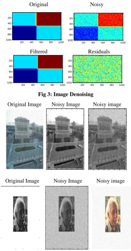
Finally in fig. 3-6, we present some qualitative results obtained by simulation using Matlab 7.0. fig. 3 shows a original and noisy image and its denoising. Fig. 4 provides
original and noisy image in gray scale and noisy image in RGB of place and Einstein.
Original Noisy
[image:3.595.323.533.97.499.2]Filtered Residuals
Fig 3: Image Denoising
Original Image Noisy Image Noisy image
Original Image Noisy Image Noisy image
[image:3.595.67.276.493.693.2]
Fig 4: Original and noisy image in grey scale and noisy image in RGB
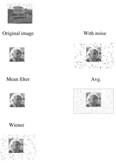
The aim of fig. 5 is to compare the quality of denoised image obtained by various denoising method by visual inspection. Fig. 6 shows the blurred image & its restoration using Non-Local Means algorithm for different NSR.
Original image With noise
Mean filter Avg.
Wiener
original
20 40 60 80 100 20 40 60 80 100 noisy
20 40 60 80 100 20 40 60 80 100 filtered
20 40 60 80 100 20 40 60 80 100 residuals
20 40 60 80 100 20 40 60 80 100 original
20 40 60 80 100 20 40 60 80 100 noisy
20 40 60 80 100 20 40 60 80 100 filtered
20 40 60 80 100 20 40 60 80 100 residuals
20 40 60 80 100 20 40 60 80 100 original
20 40 60 80 100 20 40 60 80 100 noisy
20 40 60 80 100 20 40 60 80 100 filtered
20 40 60 80 100 20 40 60 80 100 residuals
20 40 60 80 100 20 40 60 80 100 original
20 40 60 80 100 20 40 60 80 100 noisy
20 40 60 80 100 20 40 60 80 100 filtered
20 40 60 80 100 20 40 60 80 100 residuals
20 40 60 80 100 20
Original image With noise
Mean filter Avg.
Wiener
[image:4.595.68.268.70.350.2]
Fig 5: Original, noisy, mean filter, avg , wiener filter image of palace and Einstein
Original Image Simulate Blur and Noise
Restoration of Blurred, Noisy Restoration of Blurred, Noisy
Image Using NSR=0 Image Using Estimated NSR
Original Image Simulate Blur and Noise
Restoration of Blurred, Noisy Restoration of Blurred, Noisy
Image Using NSR=0 Image Using Estimated NSR
[image:4.595.319.541.73.190.2]Fig 6: Blurred image and Restoration of blurred image using NSR=0 and Estimated NSR
4.
RESULTS AND DISCUSSIONS
There are several transforms that do image denoising. In this paper non local means (NL-means) algorithm[5][6][7] is used. The denoised images obtained with various algorithms are shown in Fig. 5 for visual comparison. Pixel based processing is easy to perform as well as it will give accurate results in comparison to other methods. Two images have been taken in which one is available on system and the other which is taken from the digital media and then downloaded to the computer. Difference is occurred in the processing of two images i.e. the image which is already available has got aligned pixels than the image that is downloaded from the digital media.
5.
CONCLUSIONS
This paper gives a generalized method for image denoising. Then in depth talk about the non-local means algorithm[7] for removing noise from digital image was given. The based on simulation results, obtained by Matlab 7.0. Non-local means algorithm for image denoising is analyzed on place and Einstein images. Also it was shown by experimental results that the performance of the NL-means algorithm[5][6] outperforms several well-known denoising benchmarks in terms of the NSR value.
In future the matlab code can be converted to VHDL code and implemented on FPGA kit in order to develop ASIC (application specific IC) for image transformation and analysis. ASIC can be made for doing the specific work of image denoising ,so a person who don’t know any algorithm for image denoising are also capable of doing it
6.
ACKNOWLEDGMENTS
Our thanks to the experts who have contributed towards development of the template.
7.
REFERENCES
[1] Ke Lu , Ning He, Liang Li, “Non-Local Based denoising for medical images,”Computational and Mathematical methods in Medical ,vol.2012,pp.7,2012.
[2] H. Takeda, S. Farsiu, and P. Milanfar, “Kernel regression for image processing and reconstruction,” IEEE Transactions on image processing 16(2), pp. 349–366, 2007.
Image Processing (ICIP), pp. 317–320, (San Antonio, Texas, USA), Sept. 2007.
[4] A. Piˇzurica and W. Philips, “Estimating the probability of the presence of a signal of interest in multiresolution single and multiband image denoising,” IEEE Transactions on image processing 15(3), pp. 654–665, 2006
[5] A. Buades, B. Coll, and J. Morel. On image denoising methods.Technical Report 2004-15, CMLA, 2004.
[6] A. Buades, B. Coll, and J. Morel. Neighborhood filters and pde’s. Technical Report 2005-04, CMLA, 2005.
[7] A. Buades, B. Coll, and J Morel, “A non-local algorithm for imagedenoising ,” IEEE International Conference on Computer Vision and Pattern Recognition, 2005. [8] A. Buades. NL-means Pseudo-Code
http://dmi.uib.es/~tomeucoll/toni/NL-means_code.html [9] A. Efros and T. Leung. “Texture synthesis by
nonparametric sampling.”In Proc .Int. Conf .computer Vision, volume 2, pages 1033-1038, 1999.
[10]Awate SP, Tasdizen T, Whitaker RT. Unsupervised Texture Segmentation with Nonparametric Neighborhood Statistics. ECCV. 2006:494–507.
[11] Huang J, Mumford D. Statistics of natural images and models. ICCV. 1999:541–547.
[12]Lee A, Pedersen K, Mumford D. The nonlinear statistics of high- contrast patches in natural images. IJCV. 2003; 54:83–103.
[13]Mahmoudi M, Sapiro G. Fast image and video denoising via nonlocal means of similar neighborhoods.IEEE Signal Processing Letters. 2005;12(12):839–842. [14]Portilla J, Strela V, Wainwright M, Simoncelli E. Image
denoising using scale mixtures of gaussians in the wavelet domain. IEEE Trans On Image Processing. 2003;12:1338–1351.
[15]L. Rudin and S. Osher, “Total variation based image restoration with free local constraints,” in Proc. Of IEEE International Conference on Image Processing (ICIP), 1, pp. 31–35, Nov. 1994.
[16]C. Tomasi and R. Manduchi, “Bilateral filtering for gray and color images,” in Proceedings International Conference on computer vision, pp. 839–846, 1998. [17]Mathworks. The Matlab image processing toolbox.
http://www.mathworks.com/access/helpdesk/help/toolbo x/images/
[18]B. Gustavsson. Matlab Central - gen_susan.
http://www.mathworks.com/matlabcentral/files/6842/gen _susan.m.
[19]L. S¸endur and I. Selesnick, “Bivariate shrinkage with local variance estimation,” IEEE Signal Processing Letters9, pp. 438–441, 2002.