A computational study of shock speeds in high performance shock tubes pdf

A computational study of shock speeds

in high-performance shock tubes

P.J. Petrie-Repar, P.A. Jacobs

Department of Mechanical Engineering, The University of Queensland, Brisbane, 4072, Australia Received 15 November 1996 / Accepted 3 February 1997

Abstract. This paper describes U2DE, a finite-volume code that numerically solves the Euler equations. The code was used to perform multi-dimensional simulations of the gradual opening of a primary diaphragm in a shock tube. From the simulations, the speed of the developing shock wave was recorded and compared with other estimates. The ability of U2DE to compute shock speed was confirmed by comparing numerical results with the analytic solution for an ideal shock tube.

For high initial pressure ratios across the diaphragm, previous experiments have shown that the measured shock speed can exceed the shock speed predicted by one-dimen-sional models. The shock speeds computed with the present multi-dimensional simulation were higher than those esti-mated by previous one-dimensional models and, thus, were closer to the experimental measurements. This indicates that multi-dimensional flow effects were partly responsible for the relatively high shock speeds measured in the experi-ments.

Key words: Unstructured-grids, Solution-adaptive remesh-ing, Numerical dissipation, Shock speeds, Shock tubes flow

Nomenclature, Units

A: cell area in the (x,y)-plane, m2

a: temperature dependent function within Redlich-Kwong equation of state, m5/kg·s2

a0: constant within Redlich-Kwong equation of state,

m5_/kg·s2

b: constant within Redlich-Kwong equation of state, m3_/kg

CS: contact surface

Cv : specific heat at constant volume, J/kg·K E: total energy (internal + kinetic), J/kg e: specific internal energy, J/kg

F: array of flux terms

Correspondence to: P.A. Jacobs

n: unit normal vector P: pressure, Pa

Q: array of source terms R: specific gas constant, J/kg·K S: surface

T: temperature, K

TC: critical temperature, K TR: reduced temperature t: time, seconds

U: array of conserved quantities u: flow velocity, m/s

u: flow speed in x-direction, m/s v: flow speed in y-direction, m/s α: noise filter coefficient ρ: density, kg/m3 γ: ratio of specific heats σ: Courant number ϑ: cell volume, m3

ϑ0_{: volume per radian for an axisymmetric cell, m}3

Subscripts and superscripts L: left

R: right

1: driven-gas initial state 4: driver-gas initial state n: time level

1 Introduction

Shock tunnels and expansion tubes are used to generate high energy flows for the ground testing of hypersonic vehicles. Flow in each facility is usually initiated by the rupture of a primary diaphragm that separates a high pressure driver gas and a low pressure driven gas. High pressure driver gas expands into the driven section, compressing and accelerat-ing the lower pressure driven gas. A shock wave develops within the driven gas and propagates along the shock tube. The strength of shock wave which is measured by the pres-sure ratio or shock speed determines the flow conditions behind the shock and subsequently in the test section.

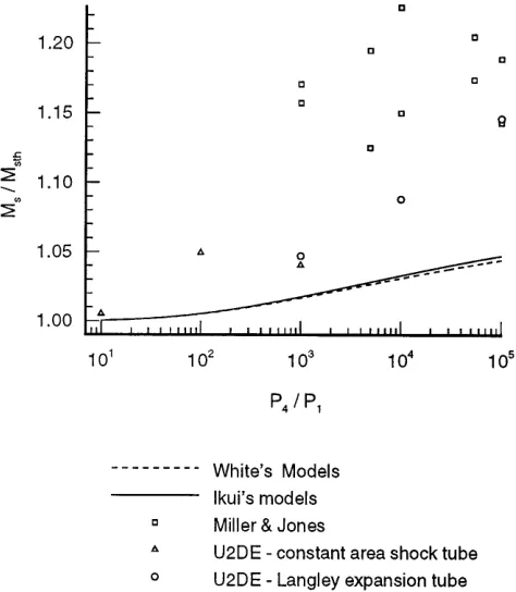
Fig. 1. Maximum Mach number of developed shock wave in a shock tube versus initial pressure ratio. Experimental data by Miller and Jones (1975) is compared with the theories of White (1958) and Ikui et al. (1969). The Mach number of the shock wave has been normalized by the Mach number of the shock wave in an ideal shock tube for the same initial conditions

can be determined by solving the unsteady one-dimensional Euler equations. The ideal shock speed has been reported by Duff (1959), to overestimate the shock speed in long, thin driven tubes where viscous effects are significant. Con-versely, measured shock speeds (White 1958; Miller and Jones 1975; Huber 1958; Nagamatsu et al. 1959; and Whit-field et al. 1966) in “high-performance” and larger diameter shock tubes can exceed the ideal shock speed by up to 20% when the initial pressure ratio across the diaphragm exceeds 103 _{as shown in Fig. 1. The higher-than-ideal shock speeds}

can be partially explained by considering the wave processes which occur during the gradual opening of a diaphragm.

1.1 Previous work

White (1958) developed a theory based on shock formation from compression waves. The model assumes that unsteady isentropic compression waves are formed in the driven gas as the diaphragm gradually opens. The compression waves are then assumed to coalesce into a shock wave at some distance downstream from the diaphragm. An upstream-facing expan-sion is formed to match the flow conditions. This model can predict higher maximum shock speeds than the ideal shock tube model, but it fails to predict the shock front acceler-ation which has been observed in experiments. As an im-provement to the model of White (1958), Ikui et al. (1969) developed a multi-stage model. They assumed that a series

of compression waves produced by the gradual opening of the diaphragm, can be divided into a finite number of groups of compressions. A group of compression waves coalesce at the same point and the shock front generated by the first group is successively accelerated by the other groups. This model can predict slightly higher maximum shock speeds than the model of White (1958) as shown in Fig. 1.

Zeitoun et al. (1979) performed a one-dimensional com-putation using the method of characteristics, in which the finite opening time of the diaphragm and boundary layer ef-fects were taken into account. The finite opening time of the diaphragm was found to induce a strong shock acceleration followed by a slow deceleration, and the maximum com-puted shock speed was close to the value predicted by the theory of White (1958). When the effects of the boundary layer were neglected, the shock still decelerated after the initial acceleration but its velocity remained higher than the ideal shock speed. However, the inclusion of boundary layer effects caused a monotonic decrease in the shock speed to the value below the ideal shock speed.

Miller and Jones (1975) measured shock-wave veloci-ties in the Langley six-inch diameter expansion tube. Air, argon, carbon dioxide and helium were used as test gases. The driver gas was always helium. The shock speed mea-surements were made using a microwave interferometer and via the response of pressure transducers positioned along the driven section (time of arrival gauges). The maximum shock speeds measured exceeded the maximum shock speeds pre-dicted by the one-dimensional theories of White (1958) and Ikui et al. (1969) at high initial pressure ratios for all test gases except argon.

The experimental work of Miller and Jones (1975) was chosen to be the reference point, because of the high quality and detail of the available experimental data. Figure 1 com-pares the normalised maximum shock Mach number (helium as the test gas) with the theories of White (1958) and Ikui et al. (1969) in which constant area tube and ratio of spe-cific heats γ = 1.667 are assumed. The maximum shock Mach number is normalised by the shock Mach number ex-pected in an ideal shock tube at the same conditions. Two important observations can be made from Fig. 1: (i) the ex-perimental data points are significantly higher than estimated values from the one-dimensional theories; and (ii) the nor-malized shock Mach number predicted by the theories of White (1958) and Ikui et al. (1969) increases with initial pressure ratio.

Miller and Jones (1975) suggested that the higher shock speeds were caused by a combination of mechanisms in-cluding heating of driver gas during pressurisation, effects of the finite opening time, and multi-dimensional effects. The multi-dimensional nature of the flow resulting from a gradually opening diaphragm is examined here to determine if it contributes significantly to the higher-than-expected ex-perimental shock speeds.

Fig. 2. Interpolation geometry

Fig. 3. Geometry associated with error function

wall. Most of the work concentrated on the flow develop-ment and, in particular, on the structure of contact surface and the expansion waves in the driver gas.

Satofuka (1970) performed a numerical study of shock formation in cylindrical and two-dimensional shock tubes. Air/Air driver-driven gas combinations were examined at diaphragm pressure ratios of 10, 100 and 1000. The calcu-lated shock speeds were similar to those of White (1958) and Ikui et al. (1969) at the lower initial pressure ratios. However, at the highest pressure ratio of 1000, a slightly higher shock speed (+0.05%) was predicted.

Outa et al. (1975) performed experiments and two-dimensional simulations of a gradually opening diaphragm. From schlieren pictures and the numerical simulations, the presence of oblique shock waves interacting with a two-dimensional unsteady expansion was observed. It was con-cluded that the effects of these waves on the flow structure were restricted to one to two diameters downstream. The maximum experimentally measured shock speed within a 100 mm square shock tube for an initial pressure ratio of 6100 exceeded the ideal shock speed by 10% and exceeded the maximum shock speed predicted by the theory of Ikui et al. (1969) by 5%.

Cambier et al. (1992) performed a two-dimensional ax-isymmetric simulation of gradual diaphragm rupture in which the diaphragm was modelled as an opening iris. The fol-lowing observations were made from the simulations; the primary shock becomes planar very rapidly (within two di-ameters from the diaphragm), a complex and unsteady flow structure dominated by a Mach disk is formed behind the contact surface (CS), and the CS itself becomes a complex

shape. The initial shape of the CS is due to the relatively slow opening time of the diaphragm. The contact surface CS does not become planar with time, and it was suggested that its fate could be dominated by Rayleigh-Taylor instabilities. Vasil’ev and Danil’chuk (1994) performed an inviscid two-dimensional simulation of shock wave formation in a shock tube by considering transverse diaphragm removal. Two main observations were made from their simulations: (i) jetting of the CS along the walls due to a system of oblique shock waves; and (ii) fragmentation of the secondary shock which occurred because a pocket of hot unexpanded gas at the wall changed the effective area of the tube. The resulting flow is analogous to the flow through a Laval nozzle.

1.2 Scope of the current work

The results from two-dimensional axisymmetric simulations of a gradually opening diaphragm with high initial pressure ratios are presented here. The simulations were performed using a finite-volume code, U2DE, which solves the Euler equations. The diaphragm opening is modelled as an iris, similar to the model proposed by Cambier et al. (1992). Particular attention is directed to the variation of the speed of the developing shock.

Experimental conditions approximating those reported by Miller and Jones (1975) were investigated. The mod-els of White (1958) and Ikui et al. (1969) fail to predict the maximum shock speed at these conditions. It will be shown that the multi-dimensional nature of flow contributed to the higher than expected maximum shock speed. The structure of the flow as it developed during and after diaphragm rup-ture, and in particular the contact surface, are also examined.

2 Computational model

A cell-centred finite-volume code, U2DE was used to solve numerically the Euler equations. The flow domains were represented as unstructured meshes of triangular cells and solution-adaptive remeshing was used to focus computa-tional effort in regions where the flow-field gradients were high.

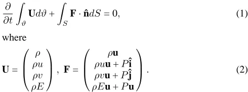
The two-dimensional Euler equations can be written as, ∂

∂t Z

ϑ Udϑ+

Z

S

F·ˆndS= 0, (1)

where U =    ρ ρu ρv ρE   , F =

  

ρu ρuu +Pˆi ρvu +Pˆj ρEu +Pu

 

. (2)

The two-dimensional cells are assumed to have unit depth. The axisymmetric form of the Euler equations can be written similarily as,

∂ ∂t

Z

ϑ0

Udϑ+ Z

Sy

F·ˆndS= Q, (3)

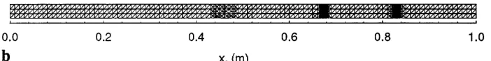
Fig. 4a,b. Initial mesh: a for ideal shock-tube problem (P4/P1 = 10) and a solution-adapted mesh; b at timet= 6×10−4 s

Q =   

0 0 P A

0  

. (4)

The volume of the cell is expressed as volume per radian (ϑ0).

For calorically perfect gas, the equation of state of ideal gas is used,

P = (γ−1)ρe. (5)

The specific internal energy is written as,

e=E−1 2(u

2_+v2_{). (6)}

However, the initial pressure of the helium driver gas used by Miller and Jones (1975) was high enough to cause devi-ation from ideal gas behaviour due to van der Waals forces. The Redlich-Kwong equation of state (Aungier 1995) can be used in (7) to describe more accurately the behaviour of helium at the flow conditions of interest.

P = ρRT 1−bρ +

ρ2_a(T)

1 +bρ, (7)

a(T) =a0T_R−0.03, (8)

TR= _TT

c, (9)

T = e

Cv, (10)

wherea0= 226.20 m5/kg·s2,b= 4.1648×10−3 m3/kg,Cv=

3115.6 J/kg·K,R= 2077 J/kg·K andT_c= 5.3 K. The specific heatC_v, was assumed to be constant.

The Euler equations are applied to each triangular cell in the discretised form,

dU dt ≈

1 ϑ

3

X

k=1

(FdS+ Q), (11)

and, from known initial conditions, the flow solution in each cell is explicitly updated in time. Each time-step can be split into three parts. Firstly, the pseudo-left and -right edge flow states are determined at the edges that bound each triangular cell. Secondly, the flux array F at each edge is determined. Finally, the cell-averaged conserved quantities U and the primary flow variables for each cell are updated.

The pseudo-left and -right edge flow states are recon-structed from the cell averaged data with each primary flow variable being treated independently. For example, the left and right edge densities (ρ_L0,ρR0) are constructed from the

densities at four nearby points (ρ_L2,ρ_L1,ρ_R1,ρ_R2) as shown in Fig. 2. If the edge is internal to the flow field,ρ_L2equals

the density at the vertex of the left cell which is opposite the edge,ρ_L1equals the density at the centre of the left cell,

ρR1equals the density at the centre of the right cell, andρR2

equals the density at the vertex of the right cell opposite to the edge. A primary flow variable at a vertex is determined by summing the primary flow variable of the surrounding cells multiplied by a weight, and then dividing by the sum of the weights. The weight is equal to the inverse of the distance from the vertex to the centre of the cell (Batina 1993).

If the edge is external, the cell associated with the edge is defined to be the right cell. The density, pressure and internal energy of the left and far-left pre-interpolation values are set to the right and far-right cell values respectively. The left and far-left velocities are set to the reflected velocities of the right and far-right cell respectively with the edge acting as a mirror.

To model the gradual opening of the diaphragm, U2DE has the ability to blank out (ignore) parts of the domain. The use of unstructured meshes made the implementation of this feature easy. Edges between an ignored cell and a flow cell are treated as a wall.

A generalized MUSCL interpolation scheme (Anderson et al. 1985) is used to construct the left and right flow states from the pre-interpolation flow states as

ρL0=ρL1+∆L,

ρR0=ρ_R1+∆_R, (12)

where

∆L = 1₄[(1−κ)MM{(ρL1−ρL2), β(ρR1−ρL1)}

+(1 +κ)MM{β(ρ_L1−ρL2),(ρR1−ρL1)}],

∆R =−1₄[(1 +κ)MM{(ρR1−ρL1), β(ρR2−ρR1)}

+(1−κ)MM{β(ρ_R1−ρL1),(ρR2−ρR1)}]. (13)

The minmod (MM) limiter function returns the argument with the minimum magnitude if both arguments have the same sign and returns zero otherwise. The parameterκ= 1/3 was used giving an upwind-biased third-order interpolation scheme, and a compression parameterβ= 2 was used.

Fig. 5a–c. Comparison of numerical density profiles for an ideal shock-tube problem (P4/P1 = 10) with analytical solution att=

600µs: a first order solution; b higher order solution; and c higher order solution with solution-adaptive remeshing

EFM becomes an upwind scheme. The EFM flux calculation assumes perfect gas. For a non-perfect gas, an effective ratio of specific heats (14) calculated from the pseudo left and right edge flow states is used (Edwards 1988).

γav = √_ρ

LγL+√ρ_Rγ_R √_ρ

L+√ρ_R , (14)

γi= _ρPi

iei + 1. (15)

The increment in flow time for each time-step is determined during the flux calculations and is equal to,

∆t=σ×minimum

local wave speed smallest cell median

, (16)

whereσ, is the Courant number and is usually set to 0.5. The cell averaged conserved quantities are advanced from time level n to time level n+ 1 using the predictor-corrector scheme

∆U(1)=∆tdU

(n)

dt , U(1)= U(n)+∆U(1), ∆U(2)=∆tdU

(1)

dt , U(n+1)= U(1)+1

2(∆U

(2)_−∆U(1)_{), (17)}

where the superscripts (1) _and (2) _{indicate intermediate}

re-sults. If a first order scheme is desired, only the first stage is used and U(n+1)= U(1).

2.1 Solution-adaptive remeshing

Solution-adaptive remeshing concentrates the computational effort at regions of interest within the flow domain. This al-lows better resolution of discontinuities such as shock waves and slip lines than would be possible with fixed-grid simu-lations at the same (or similar) computational expense. The resolution of the mesh is increased by introducing nodes to the mesh thereby increasing the number of cells in that re-gion. The resolution of the mesh can be reduced in regions where the solution has become smooth by removing previ-ously inserted nodes.

The remeshing process comprises three stages: firstly, the “error indicator” is calculated for each cell and cells are marked for deletion, refinement or no action; the second step is the deletion of vertices surrounded by cells which have been marked for deletion; and finally, cells marked for refinement are split. The frequency of remeshing depends on the Courant number and the number of “protective layers” provided during refinement. A protective layer is formed by refining the cells adjacent to the cells marked for refinement. For a Courant number σ = 0.5 and using one protective layer, remeshing was performed every five time-steps.

The primary flow variable used to calculate the error indicator is density. The error indicator associated with each cell is determined by

error indicator =nX i,j,k

|2b−a_i−c_i| o.

nX

i,j,k

(|b−a_i|+|c_i−b|) +αX i,j,k

(a_i+ 2b+c_i) o

. (18)

The geometry associated with this equation is shown in Fig. 3 wherea_iis the density at the centre of an adjacent cell, bis the density at the centre of the cell, andc_iis the density at the vertex opposite to the adjacent cell. This indicator is based on similar error functions developed by L¨ohner (1987) and Probert et al. (1991).

deletion. If the volume of a cell is lower than the specified minimum volume or area for axisymmetric cases, it is not marked for refinement.

The bisection method (Rivara 1984) is used to refine the triangular cells. Cell refinement is achieved by inserting a new vertex at the midpoint of an edge and splitting the cells adjoining the edge. The edge chosen to be split must have the greatest length of all the edges of the two cells adjoining the edge. A refinement level is assigned to a vertex when it is inserted. This number is equal to the highest refinement level of the surrounding vertices plus one. Initially the refinement level of all vertices is zero.

Only vertices associated with four or two cells (boundary vertex) are considered for deletion. All the cells connected to the vertex must be marked for deletion and the refinement level of the vertex must be higher than all vertices connected to the vertex being considered for deletion. When a vertex is inserted, the index numbers of the vertices of the split edge are stored within the data structure of the new vertex. This information is used to ensure that deletion is the reverse of a previous insertion. The retention of the local mesh allows for further vertex removal.

The cell refinement for the axisymmetric simulations was carried out in a manner so that cell aspect ratio was main-tained throughout the simulation. “Numerically induced jet-ting” along the axis has been previously observed in ax-isymmetric simulations by Cambier et al. (1992), and by the authors. Stretching the cells in the radial direction can alle-viate this problem. A cell aspect ratio of three was used for all the axisymmetric simulations presented here.

3 Code validation - ideal shock tube

The accuracy of U2DE was validated by comparing nu-merical solutions for an idealised shock tube to the one-dimensional analytical solution.

Firstly, we examine a shock tube with a low initial pres-sure ratio across the diaphragm (Hirsch 1990). The gas is assumed to be calorically perfect with γ = 1.4. The initial state at timet= 0 is

x≤0.5 m :ρ4= 1.0 kg/m3,

P4= 105Pa, u4=v4= 0,

x >0.5 m :ρ1= 0.125 kg/m3,

P1= 104Pa, u1=v1= 0. (19)

Figure 4 shows the initial mesh and a solution-adapted mesh at a later time. Profiles of density from first-order and higher-order solutions generated without solution adaptive remesh-ing and a higher-order solution generated usremesh-ing solution adaptive remeshing are shown in Fig. 5. The volume of each cell within the initial mesh is 5.0×10−5_m3_{. The minimum}

cell volume was set to 1.0×10−7m3 and the coefficient of the noise filter,αin the error indicator (18) was set to 0.01. The comparisons of the numerical solutions with the analyt-ical solution demonstrate that the current algorithm provides a satisfactory solution and that the implementation of the higher order interpolation and solution adaptive remeshing does improve the accuracy of the solution.

We now examine the ability of U2DE to produce accu-rate numerical solutions when the initial pressure ratio across the diaphragm is high. The initial state at timet = 0 is set to

x≤5.0 m :P4 = 35×106Pa,

T4 = 342 K, u4= 0,

x >5.0 m :P1 = 3450 Pa,

T1 = 297.6 K, u1= 0. (20)

This condition approximates one of the experimental condi-tions used by Miller and Jones (1975), withP4/P1= 10,145,

and provides a harsher test of the code. Helium is used as driver gas as well as test gas. The high pressure of the driver gas (x ≤ 5.0 m) leads to significant deviation from the perfect-gas model and so the Redlich-Kwong equation of state is used.

Two-dimensional planar simulations were performed. The volume of each cell within the initial mesh was 2.0× 10−4 m3. The minimum cell volume for the simulation was set to 1.0 ×10−6 _m3 _{and α = 0.01. Figure 6 compares}

the higher order numerical density profile with the one-dimensional analytical solution. The agreement is satisfac-tory but the shock position does appear to be incorrectly es-timated. Thus, the accuracy of U2DE to compute the shock speed was examined in more detail.

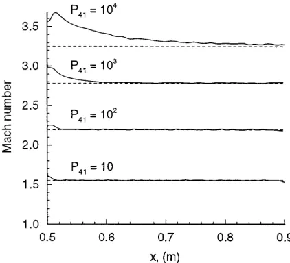
The shock speed was computed by recording the po-sition of the shock wave every ten time-steps. This data was smoothed and then differentiated. Speeds of developing shocks were computed at various initial pressure ratios (10, 100, 1,000, and 10,000) across the diaphragm and compared to the corresponding analytical shock speeds in Fig. 7. The density and pressure on the right side of the tube was set to unity. The initial temperature of the driver and driven gas was the same for all cases and the gas was assumed to be calorically perfect with γ = 1.667. The simulations used the same domain and initial mesh as the first shock tube problem as seen in Fig. 4. The minimum cell volume was set to 1.0×10−7 m3 andα= 0.03. At the lower initial pressure ratios the agreement between the computed shock speed and correct (analytical) shock speed is good. At higher initial pressure ratios, there is an initial overestimation, but the computed shock speed does decay to the correct shock speed. The magnitude of the initial overestimation and the distance required to decay to the analytical value increases with initial pressure ratio.

It was speculated that the initial overestimation of shock speed when the initial pressure is high is due to numerical diffusion, particularly at the contact surface. A test case was designed such that the initial pressure ratio across the di-aphragm was high (104_{), and the densities on either side of}

the contact surface were equal. The domain and initial mesh for the first shock tube problem as seen in Fig. 4 were used. The initial condition was,

x≤0.5 m :ρ4 = 11.9969 kg/m3,

P4 = 104Pa,

x >0.5 m :ρ1 = 1.0 kg/m3,

Fig. 6. Density profile for an ideal shock tube (P4/P1 = 10,145)

att= 500µs. Comparison of numerical solution with analytical

Fig. 7. Shock Mach number versus distance from diaphragm for an ideal shock tube. Numerical values at various initial pressure ratios are compared with analytical values. Note the diaphragm location is atx= 0.5 m

Note that this initial condition is extreme due to high initial temperature ratio and the large shock Mach number in Table 1.

Figure 8 compares the computed density profile with the analytical solution at t= 8.7 ms. The position of the shock wave agrees with the analytical position and the distance required for the shock speed to settle to the analytical speed is significantly reduced as shown in Fig. 9.

The computed shock speed versus distance from the di-aphragm for the experimental condition stated above was compared to the analytical shock speed as seen in Fig. 10. The speed of the developing shock was computed at differ-ent mesh resolutions (that is, minimum cell volume). The distance required for the shock speed to decay to the analyt-ical shock speed decreased with increasing mesh resolution (lower minimum cell volume). This is consistent with the reduction in numerical diffusion that is expected with in-creased mesh resolution. The solution adaptive remeshing

procedure is therefore an important component of the code when trying to estimate accurately the shock speeds of a high performance shock tube. The overestimation of the pri-mary shock speed by the fixed-grid Navier-Stokes code can be seen in a previous study of the NASA Langley expansion tube by Jacobs (1994) as seen in Fig. 7.

4 Simulation of gradual diaphragm opening

Numerical simulations of flow through a gradually open-ing primary diaphragm are now presented. The geometry of the domain is based on the NASA Langley expansion tube (Miller and Jones 1975) operated with the primary di-aphragm only. The diameter of the driver section was 165.1 mm and its length was 2.44 m. The diameter of the driven tube was 152.4 mm. The transition from driver tube diam-eter to driven tube diamdiam-eter occurred after the diaphragm location and extended over a length of 190.5 mm. Although the diaphragm section was square in cross-section and the transitional area change piece went from square to circular, the geometry for the current simulations was assumed to be axisymmetric.

Three experimental conditions used by Miller and Jones (1975) were examined in Table 2. The initial driver gas state,

x≤2.44 m :P4= 35×106Pa,

T4= 342 K, u4=v4= 0, (22)

was the same for all conditions. Both driver and driven gases were helium and the Redlich-Kwong equation of state was used to describe the gas behavior. The diaphragm opening was modelled as a dilating iris with an opening time of 200 µs. The minimum cell area, in the (x, y)-plane, of the initial mesh was 9.26×10−4 _m2_{, except at the diaphragm}

section. The diaphragm was created by refining the cells at the diaphragm location until the cell area was less than 5.0×10−7 _m2_{. A thin strip of cells, 4.24 mm thick was}

chosen to represent the diaphragm. These cells were initially ignored. During the simulation, the status of the ignored cells was changed to flow cells so that the flow area open was proportional to the elapse of time from its opening. The minimum cell area for the simulation was set to 5.0×10−7

m2 _{andα= 0.02.}

4.1 Flow development

The time history of the density and pressure contours for the Langley expansion tube (P4/P1 = 10,145) is shown in

Figs. 11–13. The initial shape of the shock wave is spher-ical until it reflects at the tube wall. The shock front and the reflected (transverse) waves interact causing the shock front to become planar within a relatively short distance and the transverse waves become weaker. These observa-tions of the shock front formation are similar to those made from previous numerical (Cambier et al. 1992; Vasil’ev and Danil’chuk 1994) and experimental work (Henshall 1957; cited by Miller and Jones 1975).

Table 1. Summary of test cases at various initial pressure ratios where the temperatures on either side of the diaphragm are equal unless specified otherwise

Pressure Shock Contact surface Flow CPU Final number Time ratio Mach number density ratio time (s) (s) of cells steps

10 1.5520 2.5942 0.20 702 2,029 3,393

100 2.1945 7.3295 0.14 3,685 7,552 3,490

1,000 2.7844 21.153 0.11 6,615 11,089 3,517

10,000 3.2491 59.473 0.095 9,565 16,515 3,640

10,000a _{35.611 1.0000 0.0087 788 1,954 3,539}

a _{Initial temperature ratio is 833.55}

Fig. 8. Ideal shock tube with a high initial pressure ratio (104_{), but}

with no contact surface discontinuity. Comparison of numerical solution (◦) with analytical solution (dashed line) at t= 8.7 ms. Minimum cell volume of 1.0×10−7 m3andα= 0.01

Fig. 9. Computed shock Mach number (solid line) versus distance compared with analytical Mach number (dashed line) for an ideal shock tube with high initial pressure ratio of 10,000 but no contact surface discontinuity. Note the diaphragm location is atx= 0.5 m

Fig. 10. Shock speed versus distance from diaphragm for an ideal shock tube. The initial condition is the same as an experimental condition of Miller and Jones (1975). Computed speeds at vari-ous mimimum cell volumes (m3) are compared with the analytical speed

of the tube. At approximately 100 µs the interaction of the radially expanding driver gas with the tube wall causes an oblique upstream-facing shock to develop. This shock redi-rects the flow along the wall and causes the density and the pressure of the flow behind the contact surface to be higher at the wall than at the central part. This region of higher pressure gas accelerates the contact surface at the wall rel-ative to the centre. The contact surface eventually becomes concave when viewed from the downstream end. The evolu-tion of the contact surface is similar to that observed in the previous numerical studies. Note that the study of Cambier et al. (1992) took into account viscous effects which slowed down the contact surface at the walls, but the jetting of the contact surface near the walls relative to the center of the tube was evident.

Fig. 11. Time history at 20 – 80 µs of density (top) and pres-sure (bottom) contours for the numerical simulation of the primary diaphragm opening within the NASA Langley facility

4.2 Shock speed

The computed shock speeds as functions of distance down-stream from the diaphragm for the initial conditions stated in Table 2 are compared with the experimentally measured shock speeds shown in Fig. 14. The maximum experimen-tal shock speeds exceed the computed speeds for all cases, however, the experimental and computed profiles are simi-lar in that both exhibit an acceleration phase followed by a deceleration phase. Note that the computed profile has a

de-Fig. 12. Time history at 100 – 160µs of density (top) and pres-sure (bottom) contours for the numerical simulation of the primary diaphragm opening within the NASA Langley facility

celeration phase even though viscous effects are not included which was also noted by Zeitoun et al. (1979).

The grid convergence of the computed shock speeds was examined in Fig. 15, and only occurred forP4/P1 = 1014.5.

This is similar to results for the ideal shock tube as dis-cussed in Section 3, where the shock speed converged to the ideal value for P4/P1 ≤ 1,000. The simulation with

the highest mesh resolution forP4/P1= 10,145 required 22

days of computation time (on a SGI R8,000 processor; 85µs per cell per predictor-corrector time-step) and a higher res-olution simulation could not be obtained with the available computing resources.

Due to the uncertainty of the computed maximum shock speed when the initial pressure ratio was high, axisymmetric simulations of gradual diaphragm opening were performed at lower initial pressure (10, 100, 1,000) ratios. The simu-lations were for a constant diameter tube (152.4 mm) with a diaphragm opening time of 200µs. The gas was assumed to be perfect helium (γ= 1.667). The driven gas fill condi-tion wasρ1= 1.0×10−3kg/m3, P1= 623.1 Pa. The driver

gas and driven gas were assumed to have the same initial temperature (300 K).

Fig. 13. Time history at 180 – 240 µs of density (top) and pres-sure (bottom) contours for the numerical simulation of the primary diaphragm opening within the NASA Langley facility

in Fig. 16. Grid convergence was only achieved forP4/P1=

1000. For P4/P1 = 10 and 100 the difference between the

highest and middle resolution is greater than the difference between the middle and lowest resolution. However, the changes are small for P4/P1= 10. The reason for this is

presently unknown, but we suspect numerical jetting, which has been demonstrated to become worse for higher resolu-tion axisymmetric simularesolu-tions (Cambier et al. 1992).

The maximum shock speed can occur within half a me-tre downsme-tream of the diaphragm location as seen in Fig. 16. This is due to the interaction of the spherical shock wave with the shock tube wall. The maximum shock speed re-ferred to by this paper is the maximum developed shock speed after the shock has become planar and initial tran-sients have settled.

The maximum shock speeds for the simulations of grad-ual diaphragm opening are compared to theoretical and ex-perimental shock speeds as seen in Fig. 1. Note that grid convergence was only achieved for P4/P1 = 1,000 and

1014.5. Despite this, the trend is consistent; the shock speed in the axisymmetric shock tube with a gradually opening diaphragm is greater than the speed predicted by various one-dimensional theories (White 1958; Ikui et al. 1969) for the same initial conditions. It is believed that this is related to the oblique upstream facing shock that temporarily appears downstream of the diaphragm which raises the entropy of the driver gas. Zeitoun et al. (1979) showed, using a one-dimensional model that, if an upstream facing normal shock exists downstream of the expansion, the speed of the shock wave can transiently exceed the ideal value. The theories of White (1958) and Ikui et al. (1969) do not consider this up-stream facing shock. The idea of increasing the entropy of the driver gas to generate faster shocks has been studied by Bogdanoff (1990) and Kendall et al. (1996), and it appears that similar entropy raising mechanisms are operating here.

Fig. 15a–c. Computed shock speeds within NASA Langley expan-sion tube assuming gradual diaphragm opening. The shock speeds were computed from simulations at various minimum cell areas (m2_{). The initial pressure ratios are: a 1014.5; b 10,145; and c}

101,450

The computed shock speeds obtained via the multi-dimensional model, although higher than the one-dimension-al shock speeds, are less than the experimentone-dimension-al vone-dimension-alues of Miller and Jones (1975). There are a number of possible reasons for this. The simulations did not include the viscous and turbulent mixing that occurs at the contact surface. The temperature of the expanded gas can be very low (16 K for

Fig. 16a–c. Computed shock speeds in a constant area shock tube with gradual diaphragm opening: aP4/P1 = 10; bP4/P1 = 100;

and cP4/P1 = 1,000. The Mach number of the shock wave has

Table 2. Pressure and temperature of driven gas and maximum shock speeds from experiments by Miller and Jones (1975). The driver conditions wereP = 35 MPa andT = 342 K

Pressure (kPa) Temp (K) Max shock speed (m/s)

34.5 297.0 3,490

3.45 297.6 4,206

0.345 297.6 4,511

P4/P1= 1,000), and at these temperatures, the behaviour of

the gas cannot be considered ideal. Also the opening of the primary diaphragm via petaling is fully three-dimensional and the current simulation is not modelling this process fully. As a final note, it has been shown that numerical diffu-sion does affect the computed shock speed for shock tube simulations whenP4/P1>1,000. Considering this, the

dif-fusive EFM flux calculator may appear to be a poor choice. However, an approximate Riemann solver (Jacobs 1992) which is less dissipative was also tried. When the initial pressure was high, this less dissipative method generated unacceptable levels of noise in the solution, particularly be-hind the shock. This phenomena, may be related to odd-even decoupling as discussed by Quirk (1994).

5 Conclusion

The finite-volume code U2DE solves the Euler equations for compressible flow and can be used to model shock tube flow and accurately compute shock speeds when the initial pres-sure ratio is low. When the initial prespres-sure ratio is high the flow is difficult to resolve because of the large density ratio at the contact surface where significant numerical diffusion occurs. However, solution-adaptive remeshing can be used to control the error and obtain reasonable estimates for the shock speed.

Axisymmetric simulations of the flow through a slowly-opening diaphragm were performed. The structure of the developing flow was similar to flows observed by previous experimental and numerical work, and the maximum speeds of the primary shock wave for the multi-dimensional simu-lations of diaphragm opening exceeded the speeds predicted by previous one-dimensional theories (White 1958; Ikui et al. 1969). It is possible that one of the mechanisms behind the increase in the shock speed is an entropy rise through the oblique shock structure which exists temporarily down-stream of the diaphragm while it is opening. The mechanism is a multi-dimensional flow effect that can be captured only in two- or three-dimensional simulations.

Acknowledgements. The computer simulations were run on the

University of Queensland High Performance Computing Facility.

References

Anderson WK, Thomas JL, Van Leer B (1985) A comparison of finite volume flux vector splitting the Euler equations. AIAA Paper 85-0122

Aungier RH (1995) A fast, accurate real gas equation of state for fluid dynamic analysis applications. J of Fluids Eng 117:277

Batina JT (1993) Implicit upwind solution algorithms for three-dimensional unstructured meshes. AIAA J 31:801

Bogdanoff D (1990) Improvements of pump tubes for gas guns and shock tube drivers. AIAA J 28:383

Cambier JL, Tokarcik S, Prabhu DK (1992) Numerical simula-tions of unsteady flow in a hypersonic shock tunnel facility. In: AIAA 17th Aerospace Ground Testing Conference, Nashville, TN

Duff RE (1959) Shock-tube performance at low initial pressure. Phys Fluid 2:207

Edwards TA (1988) The effect of exhaust plume/afterbody inter-action on intalled scramjet performance. Tech Rep 101033, NASA Technical Memorandum

Henshal BD (1957) On some aspects of the use of shock tubes in aerodynamic research. Tech Rep 3044, A.R.C.

Hirsch C (1990) Numerical Computation of Internal and Exter-nal Flows. Volume 1: ComputatioExter-nal Methods for Invisid and Viscous Flows. J Wiley and Sons

Huber PW (1958) Note on hydrogen as a real-gas driver for shock tubes. J Aeronautical Sciences :269

Ikui T, Matsuo K, Negi M (1969) Investigations of the aerodynamic characteristics of the shock tubes. Bulletin JSME 12:783 Jacobs PA (1992) Approximate Riemann solver for hypervelocity

flows. AIAA J 30:2558

Jacobs PA (1994) Numerical simulation of transient hypervelocity flow in an expansion tube. Computer Fluids 23:77

Kendall MA, Morgan RG, Jacobs PA. A compact shock-assisted free-piston driver for impulse facilities. (Accepted for publica-tion in Shock Waves)

L¨ohner R (1987) An adaptive finite element scheme for tran-sient problems in CFD. Computer Meth in Applied Mech Eng 61:323

Macrosson MN (1989) The equilibrium flux method for the calcu-lation of flows with non-equilibrium chemical reactions. J of Comp Phys 80:204

Miller CG, Jones JJ (1975) Incident shock-wave characteristics in air, argon, carbon dioxide, and helium in a shock tube with unheated helium driver. Tech Rep TN D-8099, NASA, Langley Research Center Hampton, Va 23665

Nagamatsu HT, Geiger RE, Sheer RE (1959) Hypersonic shock tunnel. Am Rocket Soc J 29:332

Outa E, Tajima K, Hayakawa K (1975) Shock tube flow influ-ence by diaphragm opening (two-dimentional flow near the diaphragm). In: Kamimoto G (ed) 10th Int Symp on Shock Tubes pp 312–319

Probert J, Hassam O, Peraire J, Morgan K (1991) An adaptive finite element method for transient compressible flows. Int J Numerical Methods in Eng 32:1145

Pullin DI (1979) Direct simulation methods for compressible in-viscid ideal-gas flow. J Comp Phys 34:231

Quirk JJ (1994) A contribution to the great Riemann solver debate. Int J Num Methods in Fluids 18:555

Rivara MC (1984) Mesh refinement processes based on the gener-alized bisection of simplices. SIAM J Num Analysis 21:604 Satofuka N (1970) A numerical study of shock formation in

cylin-drical and two-dimensional shock tubes. Tech Rep 451, ISAS, University of Tokyo, Japan

Taylor GI (1950) The instability of liquid surfaces when accelerated in a direction perpendicular to their planes. Proc Royal Soc Lond Series A 201:192

removal. Izvestiya AN SSSR Mekhanika Zhidkosti i Gaza 2:147

White DR (1958) Influence of diaphragm opening time on shock-tube flow. J Fluid Mech 4:585

Whitfield JD, Norfleet GD, Wolny W (1966) Status of research on a high performance shock tunnel. Tech Rep AEDC-TR-65-272, US Air Force