Soft Sensor based on Adaptive Linear Network for
Distillation Process
Asha Rani
Instrumentation and Control Engineering Division NSIT, Sec-3, Dwarka, New
Delhi
Vijander Singh
Instrumentation and Control Engineering Division NSIT, Sec-3, Dwarka, New
Delhi
J.R.P Gupta
Instrumentation and Control Engineering Division NSIT, Sec-3, Dwarka, New
Delhi
ABSTRACT
The main objective in refining units is to keep the product quality within specifications in the faces of disturbances. Online measurements of product composition using composition analyser are neither easy nor economically viable. In an effort to overcome these difficulties various soft sensors are designed in the recent years. In this research work, the authors have proposed the design of neural network based soft sensor for two types of chemical processes i.e. reactive distillation process and multicomponent distillation process. The designed soft sensor is based on adaptive linear network, Adaline and is used to infer the product composition from the temperature profile of the respective processes. For a comparative study Levenberg Marquardt based artificial neural network soft sensor is also designed. It is observed from the results that the Adaline based soft sensor is more efficient in comparison to LM based ANN soft sensor in terms of accuracy, time taken for training and memory usage.
General Terms
Application of Adaptive Linear Network in distillation process.
Keywords
Adaline soft sensor, LM soft sensor, Reactive distillation
process, Multicomponent distillation.
1.
INTRODUCTION
For successful control of distillation process, the online measurement of product composition is quite important. The measurements using composition analysers are difficult because they are expensive, difficult to maintain, require frequent calibration and have undesirable time delays. Therefore to avoid such type of difficulties, the composition is predicted from secondary measurements such as temperature measurements, pressure, heat input, reflux flow etc. [1][2]. Sungyong Park and Chaonghun Han [3] proposed a design methodology to design a soft sensor for chemical processes that can handle the correlations among many process variables and nonlinearities based on smoothness concepts. Yao Wu and Xionglin Luo [4] introduced multirate data fusion technology based on Kalman filter into soft sensor maintenance, to integrate the soft sensor model estimation with process measurement. The results demonstrated that the multirate Kalman filter approach provides improved accuracy and reliability of soft estimation when essentially dynamics is included in the Kalman filtering model and the filter parameters are properly tuned. Pierantonio Facco
et al. [5] developed a moving average partial least square soft sensor for online product quality estimation in an industrial
batch polymerization process. Almila Bahar and Canan Ozgen [6] designed an ANN based estimator system and used it in the feedback inferential control algorithm. Inputs to the controller are estimated compositions from ANN and the reflux ratio information. In the control law scheduling policy is used and predefined set points are the optimal reflux ratio profile. A. Rogina et al. [7] conducted multiple linear regression analysis and used neural networks based models to develop soft sensors. The best results were obtained with multilayer perceptron and radial basis function neural networks on considering statistical and sensitivity analysis. Ming-Da Ma et al. [8] developed an adaptive soft sensor based on statistical identification of key variables. The inferential model built by the selected key variables predicted accurately and matched the real plant situation which made it useful for industrial applications. S.R.
Vijaya Raghavan et al. [9] presented the design and
implementation of a recurrent neural network (RNN) based inferential state estimation scheme for an ideal reactive distillation column. The performance of RNN shows better state estimation capability as compared to other state estimation schemes in terms of qualitative and quantitative performance
indices. L. Fortuna et al. [10] designed neural based soft sensors
to improve product quality monitoring and control in a refinery by estimating the stabilized gasoline concentration in the top flow and the butane concentration in the bottom flow of a debutanizer column, on the basis of a set of available
measurements. Fatima Barcelo-Rico et al. [11] presented a
methodology for the design of a fuzzy controller applicable to continuous process based on local fuzzy models and velocity linearization.
The present work deals with the design of two types of artificial neural network based soft sensors. The adaptive linear network is used to estimate the product composition of two distillation processes from the respective temperature profiles. The LM soft sensor based on Levenberg-Marquardt trained artificial neural network is also designed for comparison purpose [2]. The proposed sensors are discussed in the next section.
2.
PROPOSED SOFT SENSORS
2.1 Adaptive Linear Network (Adaline) Soft
Sensor
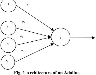
network. In Fig. 1 an input layer with x1,...,xn and bias and an
[image:2.612.81.266.108.254.2]output layer with only one output neuron is present. The input and output neurons possess weighted interconnections.
Fig. 1 Architecture of an Adaline
The output y of the Adaline is given as,
= ∑ + (1) The weights are trained using least mean square algorithm based on the use of [13] instantaneous values of cost function namely,
() =
() (2)
where e(n) is the error signal measured at time n.
Differentiating E(w) with respect to the weight vector w yield ()
= ()
( )
(3)
The algorithm operates with a linear neuron so the error signal is expressed as
() = () − ()() (4)
hence
( )
( )= −() (5)
and
()
( )= −()() (6)
using the later result as an estimate of gradient vector
() = −()() (7)
Finally using the eqn. (7) for the gradient vector in equation of weight upgradation for the method of steepest descent, the least mean square algorithm is formulated as
( + 1) = () + ()() (8)
where, is the learning rate parameter.
In this paper single layer Adaline network is used to predict the composition of distillate product from temperature profile of the column.
2.2 Levenberg-Marquardt Soft Sensor
The Levenberg-Marquardt soft sensor is an LM trained artificial neural network. The algorithm minimizes the functions that are sums of squares of other nonlinear functions [14]. The neural
network training uses mean square error as the performance index which can be minimized using LM algorithm.
In present work the Levenberg-Marquardt algorithm is applied to estimate the composition of multicomponent distillation process and reactive distillation process [7]. If each target occurs with equal probability, the mean squared error is proportional to the sum of squared error over the Q targets in the training set.
() = ∑ !%" "− #"$(!"− #")
= ∑%"""= ∑%"∑ (*&+ &,")= ∑ (() ) (9)
where &,"is the jth element of the error for the ,-. input /target pair.
The key step in the Levenberg-Marquardt algorithm is the computation of the Jacobian matrix. To perform this computation, a variation of back propagation algorithm is used. To create the Jacobian matrix, the computation of derivatives of the errors is needed, instead of the derivatives of the squared errors. Note that the error vector is
/= 0( (, … , ()2 = 0 , … ,
*3+,. , … , *3+,%2 (10)
The parameter vector is
5= 0 , … , )2 =
0, … , *36,7, , … , *6 , , … , *38+2 (11) The standard back propagation method calculates terms like
9 :;=
< =<
:; (12)
For the elements of the Jacobian matrix that are needed for the Levenberg-Marquardt algorithm need to calculate terms like
0>2.,?=@:A;=:B,<; (13)
Now the elements of Jacobian matrix can be computed as
0>2.,?=@:A;=CB,<D,EF=B,< D,<
F× D,<
F
CD,EF= H̃,.
J× D,<F
CD,EF= H̃,.
J × # &,"JK
(14)
or if
x
lis a biasLJ= ∑*&FM6,&J#&JK+ J, NℎPQRP D
F
CD,EF= #&
JK S
and L DF
TDF= 1S
0>2.,?=U(U. ? =
UV,"
UJ =
UV,"
U,"J ×
U,"J
UJ = H̃,. J ×U,"J
UJ = H̃,. J
(15) The Marquardt sensitivities can be computed through the same recurrence relations as the standard sensitivities (eq. 16), with one modification at the final layer. For the Marquardt sensitivities at the final layer we have
H̃,.8 =UU(. ," 8 =UUV,"
,"
8 =U !V,"− #V," 8 $
U,"8 = −
U#V,"8
UV,"8 1
x1
x2
xn
y b
w1
w2
= W−Q38 ,"
8$ QRP X = Y
0 QRP X ≠ Y\
(16)
Therefore when the input ]" are applied to the network and the corresponding network output #"8 are calculated, the Levenberg-Marquardt back propagation is initialized with
H̃"8= −38 "8$ (17)
where 38 "8$ is defined in equation (17). Each column of the matrix H̃"8 must be back propagated through the network using equation (16) to produce one row of the Jacobian matrix. The column can also be back propagated together using
H̃"J= −3J "J$(J^)H̃"J^ (18)
The total Marquardt sensitivity matrices for each layer are then created by augmenting the matrices computed for each input:
_`8= 0H̃J, H̃J, … , H̃"J2 (19)
It is to be noted that for each input presented to the network the sensitivity vectors _`8will be back propagated. This is because the derivative of each individual error is computed, rather than the derivative of the sum of squares of the errors. For every input applied to the network there will be _`8errors (one for each element of the network output).
The Levenberg-Marquardt technique derived in above section is summarized in the following steps.
Step1: Compute the error using target and actual output calculated by network. Compute the sum of squared errors for over all outputs using equation (9).
Step2: The Jacobian matrix is calculated using error with respective inputs.
Step3: The sensitivities are calculated with the recurrence relations in equation (17) initializing with the equation (16).
Step4: The individual matrices are augmented into the Marquardt sensitivities using equation (19) and compute the elements of the Jacobian matrix using equations (14) and (15).
Step5: Solve the following equation to get the value of ∆V.
∆V= −0>(V)>(V) + μVc2K>(V)d(V) (20)
Step6: Recompute the sum of squared errors using the new value
V+ ∆V. If the new sum of squares of errors is smaller than the error computed in step 1 then divide μ by e and
let V^= V+ ∆V and go back to step 1. If the sum of
squares is not reduced then multiply μ by e, and go back
to step 3.
The LM algorithm discussed above is used to update the weights of the artificial neural network and the network is then used for estimating the distillate composition.
3.
CASE STUDIES
Two cases of applications to distillation column are analysed; reactive distillation process and Multi component distillation process. The proposed soft sensors are used to estimate the product composition for the two processes.
3.1 Reactive Distillation Process
Reactive distillation is a process of chemical reaction and separation of the products in the common chamber. It is a highly nonlinear and complex process. The chemical industry prefers reactive distillation due to its high gain and compact nature. Reactive Distillation Column (RDC) is an ideal two-reactant-two-product column proposed by Al-Arfaj and Luyben [15] and later developed into state space model. It consists of a reactive section in the middle and non-reactive rectifying and stripping sections at the top and bottom respectively.
The column consists of Reactive Trays (NRX=9) in the middle, Rectifying Trays (NR=5) in the top and Stripping Trays (NS=5) in the bottom. The trays of the column are numbered from reboiler to condenser. The reaction that takes place in the reactive zone is exothermic liquid-vapour in nature and is given by
f + g ↔ i + j (21)
During the distillation process, the reactant B which is one of the input feeds is recovered in the rectifying section from the output product C whereas the second feed i.e. reactant A, is recovered from output product D in the stripping section. The reactive section comprises the middle section of the reactive distillation column where the reactants A and B react to produce C and D. The reaction generates the heat which is then used for the distillation of the products. The products are separated to prevent any undesired reaction between reactants A and B and products C and D. The volatilities of the products and reactants are such that
kl> kn> kT> ko (22) where k& is the volatility of the p-. component, p = #, , q, .
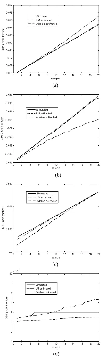
(a)
(b)
(c)
[image:4.612.79.251.74.679.2](d)
Fig. 2 Estimated composition of distillate product (a) XD1 (b) XD2 (c) XD3 (d) XD4
3.2
Multicomponent Distillation Process
The multicomponent distillation column under consideration is having 15 trays, a reboiler to vaporise the mixture and a condenser to cool the overhead vapour. Tray 5 is used as feed tray. In distillation, a liquid mixture is fed on the feed tray and the mixture is stored in reboiler. The heat is introduced in the reboiler to produce vapour. The vapour starts flowing from the reboiler to top tray and then to condenser through stripping and rectifying section. During initial start-up period, the column operates under total reflux condition in which vapour from the top of the column is condensed and returned to the column through reflux drum. During the column operation under total reflux condition, the concentration of the lightest component builds-up on the upper trays of the column and the concentrations of the intermediate component and heaviest component decreases in the top of the column but increases in the still pot. When the concentration of the lightest component in the distillate reaches its specified purity level, then the distillate product withdrawal begins.
(a)
(b)
0 2 4 6 8 10 12 14 16 18 20
0.068 0.069 0.07 0.071 0.072 0.073 0.074 0.075 0.076 0.077
sample
X
D
1
(
m
o
le
f
ra
c
ti
o
n
)
Simulated LM estimated Adaline estimated
0 2 4 6 8 10 12 14 16 18 20
0.018 0.0185 0.019 0.0195 0.02 0.0205 0.021 0.0215 0.022
sample
X
D
2
(
m
o
le
f
ra
c
ti
o
n
)
Simulated LM estimated Adaline estimated
0 2 4 6 8 10 12 14 16 18 20
0.9 0.905 0.91 0.915
sample
X
D
3
(
m
o
le
f
ra
c
ti
o
n
)
Simulated LM estimated Adaline estimated
0 2 4 6 8 10 12 14 16 18 20
-4 -2 0 2 4 6 8 10x 10
-4
sample
X
D
4
(
m
o
le
f
ra
c
ti
o
n
)
Simulated LM estimated Adaline estimated
0 5 10 15 20 25 30
9.84 9.86 9.88 9.9 9.92 9.94 9.96 9.98x 10
-3
sample
X
D
1
(
m
o
le
f
ra
c
ti
o
n
)
simulated LM estimated Adaline estimated
0 5 10 15 20 25 30
0.9895 0.9895 0.9895 0.9895 0.9896 0.9896 0.9896 0.9896 0.9896 0.9897
sample
X
D
2
(
m
o
le
f
ra
c
ti
o
n
)
(c)
(d)
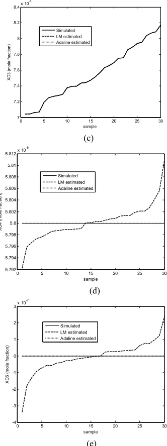
[image:5.612.84.250.75.519.2](e)
Fig. 3 Estimated Composition of Liquid composition in Distillate (a) XD1,(b) XD2, (c) XD3 (d) XD4, (e) XD5
The quality of distillate must be maintained within the specified limits which require the composition measurement. The measurements made by the composition analysers are difficult due to time delay and maintenance reasons. Therefore the product composition is measured with the help of soft sensors. In the present work two soft sensors are designed for estimation of product composition. The data used for training the soft sensors is acquired by simulating the mathematical model of multicomponent distillation process for variable heat input. In this case temperature profile (temperature of 15 trays, reboiler and condenser), heat input, reboiler pressure and reflux flow rate are used as inputs and liquid and vapour compositions of five components in distillate are the target outputs for the soft sensors. The data set so generated is used for training and testing of the designed soft sensors. The test results obtained are shown in Fig.3 and Fig.4.
(a)
(b)
(c)
(d)
0 5 10 15 20 25 30
7 7.2 7.4 7.6 7.8 8 8.2 8.4x 10
-3 sample X D 3 ( m o le f ra c ti o n ) Simulated LM estimated Adaline estimated
0 5 10 15 20 25 30
5.792 5.794 5.796 5.798 5.8 5.802 5.804 5.806 5.808 5.81 5.812x 10
-5 sample X D 4 ( m o le f ra c ti o n ) Simulated LM estimated Adaline estimated
0 5 10 15 20 25 30
-4 -3 -2 -1 0 1 2 3x 10
-7 sample X D 5 ( m o le f ra c ti o n ) Simulated LM estimated Adaline estimated
0 5 10 15 20 25 30
0.4245 0.425 0.4255 0.426 0.4265 0.427 0.4275 0.428 0.4285 0.429 sample Y D 1 ( m o le f ra c ti o n ) Simulated LM estimated adaline estimated
0 5 10 15 20 25 30
0.5715 0.572 0.5725 0.573 0.5735 0.574 0.5745 0.575 sample Y D 2 ( m o le f ra c ti o n ) Simulated LM estimated Adaline estimated
0 5 10 15 20 25 30
1.25 1.3 1.35 1.4 1.45
x 10-4
sample Y D 3 ( m o le f ra c ti o n ) Simulated LM estimated Adaline estimated
0 5 10 15 20 25 30
-1.5 -1 -0.5 0 0.5 1 1.5 2 2.5x 10
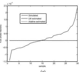
(e)
Fig. 4 Estimated vapour composition in Distillate (a) YD1,(b) YD2, (c) YD3 (d) YD4, (e) YD5
[image:6.612.87.251.76.225.2]It is observed from the estimated results that the Adaline soft sensor estimates the product composition quite accurately as compared to the LM soft sensor. In the case where the composition is very less the LM soft sensor is not able to predict the composition correctly, whereas Adaline soft sensor provides a very good estimation. It is also observed that Adaline being a single layer takes negligibly less time for training than the LM network. The memory space used, is also very less in case of Adaline network as the number of elements in the network is less. The comparison of performance parameters of the two soft sensors is shown in Table 1.
Table 1. Performance indices of estimators
Process
Estim-ator
Architecture MSE(test) Execution
time (sec)
Multi-component Distillation
Adaline 20-10 2.9092e-11 0.078
LM 20-15-15-10 1.4212e-12 88.79
Reactive Distillation
Adaline 19-4 1.9409e-8 0.016
LM 19-12-12-4 3.9629e-07 9.117
4.
CONCLUSION
In the present work, an adaptive linear network is used to design a soft sensor for estimating the product composition from temperature profile of the process. The Adaline network is similar to the perceptron but the transfer function is linear rather than hard limiting. The proposed estimator is a single layer Adaline and it uses the supervised learning algorithm known as least mean square algorithm or delta learning rule. A LM based ANN estimator is also designed for comparative study. It is observed from the results that in case of reactive distillation process the Adaline soft sensor gives more accurate results as compared to the LM soft sensor. In case of multicomponent distillation process the performance of the LM soft sensor is not up to the mark for the case where composition is very less, whereas the estimated results obtained by Adaline soft sensor coincide with the simulated composition. The Adaline soft sensor being a single layer network requires extremely less time and memory space during training. Therefore, it is concluded from the observations that the Adaline soft sensor proves to be more efficient than LM estimator in terms of accuracy, training time and memory space required for training.
Nomenclature:
=Learning parameter for neural network
rV= Eigenvalue of approximate Hessian matrix
#"= Desired qth output of the function
V,"= qth Error between target and input of kth element
s =Hessian Matrix
>()= Jacobian matrix
J =Sum of multiplication of input and weight of ith layer
H̃,.J =Marquardt sensitivity for a general layer
H̃,.8 =Marquardt sensitivity at final layer
H̃8=Total Marquardt sensitivity matrix
!"= qth target value of the function
∆V=Change in the old guess values of V
5.
REFERENCES
[1] Vijander Singh, Indra Gupta and H.O. Gupta, 2005, ANN
Based Estimator for Distillation-Inferential Control, Chemical Engineering and Processing, vol.44, Issue 7, pp. 785-795, July 2005.
[2] Vijander Singh, Indra Gupta and H.O. Gupta, 2007, ANN
Based Estimator for Distillation using
Levenberg-Marquardt Approach, special issue on Applications of
Artificial Intelligence in Process Systems Engineering, Engineering Applications of Artificial Intelligence, Elsevier Science, vol.20, pp.249-259, 2007.
[3] Sungyong Park, Changhun Han, 2000, Nonlinear Soft
Sensor Based on Multivariate Smoothing Procedure for quality Estimation in Distillation Columns, Computers and Chemical Engineering, vol.24, pp. 871-877, 2000.
[4] Yao Wu, Xionglin Luo, 2010, A Novel Calibration
Approach of Soft Sensor Based on Multirate data Fusion Technology, Journal of Process Control, vol.20, pp.1252-1260, 2010.
[5] Pierantonio Facco, Franco Doplicher, Fabrizio Bezzo,
Massimiliano Barolo, 2009, Moving average PLS Soft Sensor for online Product Quality Estimation in an Industrial Batch Polymerization Process, Journal of Process Control, vol.19, pp.520-529, 2009.
[6] Almila Bahar, and Canan Ozgen, 2010, State Estimation
and Inferential Control for a Reactive Batch Distillation
Column, Engineering Applications of Artificial
Intelligence, vol.23, pp.260-270, 2010.
[7] A. Rogina, I.Sisko, I. Mohler, Z. Uzevic, N. Bolf, 2011, Soft Sensor for Continuous Product quality estimation (in Crude Distillation Unit), Chemical Engineering Research and Design, vol.89, issue 10, Oct.2011, pp.2070-2077.
[8] Ming-Da Ma, Jing-Wei Ko, San-Jang Wang, Ming-Feng
Wu, Shi-Shang Jang, Shyan-Shu Shieh, David Shan-Hill Wong, 2009, Development of Adaptive Soft Sensor based on Statistical Identification of Key Variables, Control Engineering Practice, vol.17, pp.1026-1034, 2009.
[9] S.R. Vijaya Raghavan, T.R. Radhakrishnan, K. Srinivasan,
2011, Soft Sensor Based Composition Estimation and Controller Design for an Ideal Reactive Distillation Column, ISA transactions, vol.50, pp.61-70, 2011.
0 5 10 15 20 25 30
-1.5 -1 -0.5 0 0.5 1 1.5 2 2.5x 10
-7
sample
Y
D
5
(
m
o
le
f
ra
c
ti
o
n
)
[10]L. Fortuna, S. Graziani, M.G. Xibilia, 2005, Soft Sensor for Product Quality Monitoring in Debutanizer Distillation Columns, Control Engineering Practice, vol.13, 499-508, 2005.
[11]Fatima Barcelo Rico, Jose M. Gozalvez-Zefrilla, Jose Luis
Diez, and Asuncion Santafe-Moros, 2011, Modeling and Control of a Continuous Distillation Tower through Fuzzy Techniques, Chemical Engineering Research and Design, vol.89, pp.107-115, 2011.
[12]S.N. Sivanandam, S. Sumathi, and S.N. Deepa, Introduction
to Neural Networks using MATLAB 6.0, TATA McGraw-Hill Publishing Company Limited, New Delhi, Edition 2006.
[13]Simon Heykins, Neural Networks: A Comprehensive
Foundation, Pearson Education, Second Edition 1999.
[14]Hagan M.T., Demuth H.B., Beale M., Neural Network
Design, Vikas Publishing House, 7 International Student Edition 2003.
[15]William L. Luyben, Process Modelling, Simulation and
Control for Chemical Engineers, McGraw-Hill Publishing Company, International Edition 1996.
[16] M. A. Al-Arfaj and W. L. Luyben, Comparison of