Positive Family Functioning

(1)

Positive

Family

Functioning

29 September 2010

Final

Report

by

Access

Economics

Pty

Limited

for

Department of Families, Housing, Community

Services and Indigenous Affairs

(2)

© Access Economics Pty Limited

This work is copyright. The Copyright Act 1968 permits fair dealing for study, research, news reporting, criticism or review. Selected passages, tables or diagrams may be reproduced for such purposes provided acknowledgment of the source is included. Permission for any more extensive reproduction must be obtained from Access Economics Pty Limited through the contact officer listed for this report.

Disclaimer

While every effort has been made to ensure the accuracy of this document and any attachments, the uncertain nature of economic data, forecasting and analysis means that Access Economics Pty Limited is unable to make any warranties in relation to the information contained herein. Access Economics Pty Limited, its employees and agents disclaim liability for any loss or damage which may arise as a consequence of any person relying on the information contained in this document and any attachments.

Access Economics Pty Limited ABN 82 113 621 361 www.AccessEconomics.com.au

CANBERRA MELBOURNE SYDNEY

Level 1 9 Sydney Avenue Barton ACT 2600 Level 27 150 Lonsdale Street Melbourne VIC 3000 Suite 1401, Level 14 68 Pitt Street Sydney NSW 2000 T: +61 2 6175 2000 F: +61 2 6175 2001 T: +61 3 9659 8300 F: +61 3 9659 8301 T: +61 2 9376 2500 F: +61 2 9376 2501 For information on this report please contact Lynne Pezzullo T: 61‐2‐6175 2000 E: [email protected] Report prepared by Lynne Pezzullo Penny Taylor Scott Mitchell Laze Pejoski Khoa Le Anam Bilgrami

(3)

Contents

Acknowledgements...i

Glossary ii Executive Summary ...i

1 Introduction ... 5

2 Methodological overview ... 6

2.1 Definition of family functioning and the outcomes of interest ... 6

2.2 Data review... 7

2.3 Literature review... 10

2.4 Concepts and data underlying lifetime costing ... 10

2.5 Model construction... 11

2.6 Cost benefit/cost effectiveness analysis (CBA/CEA) and the process for selecting interventions for analysis... 18

3 Findings from the LSAC data investigation ... 21

3.1 LSAC variables ... 21

3.2 LSAC analysis... 24

4 Findings from the ATP data investigation... 31

4.1 ATP variables... 31

4.2 ATP analysis ... 34

5 The costing model... 38

5.1 Health outcomes... 38

5.2 Productivity outcomes ... 44

5.3 Criminality outcomes ... 45

5.4 Lifetime costing framework ... 49

6 Cost benefit analysis ... 52

6.1 Communities for children (CfC)... 52

6.2 Positive Parenting Program (PPP) ... 56

6.3 Reconnect ... 62

6.4 Shocking all variables – the value of PFF ... 69

7 Conclusions ... 71

References... 77

Appendix A : LSAC children and future addictive behaviours ... 85

Appendix B : Literature review sources, ATP ... 88

Appendix C : LSAC regression outcomes ... 91

Appendix D : LSAC variable specification ... 104

Appendix E : Mean and standard deviation of LSAC variables... 108

Appendix F : ATP variable interpretation... 111

(4)

Appendix H : Mean and standard deviation of ATP variables... 128

Appendix I : Detailed costing methodology and tables ... 133

Charts

Chart 3.1 : Explanatory power of regressions, by age... 26

Chart A.1 : Differences in cognitive development by socio‐economic status... 86

Tables

Table 2.1 : Characteristics of family functioning domains ... 6

Table 2.2 : FF variables used for each intervention ... 16

Table 3.1 : Regression constructs in LSAC ... 23

Table 4.1 : Regression constructs... 32

Table 5.1 : Summary of total costs of obesity (2010)... 39

Table 5.2 : Summary of total costs of anxiety and depression (2010) ... 41

Table 5.3 : Summary of total costs of daily smoking (2010) ... 42

Table 5.4 : Summary of total costs of alcohol abuse (2010) ... 43

Table 5.5 : Summary of total costs of illicit drug use (2010)... 44

Table 5.6 : Estimated effects* (%) of year 12 and undergraduate completion* on probability of participation and average earnings ... 45

Table 5.7 : Social costs of crime by cost type (2010) ... 46

Table 5.8 : Net recurrent expenditure on criminal courts (2008‐09) and % criminal court finalisations by court type ... 47

Table 5.9 : Total real net operating expenditure on prisons and community corrections in Australia in 2008‐09... 48

Table 5.10 : Discounted lifetime costs of adverse health outcomes (a) (2010 dollars)... 49

Table 5.11 : Discounted lifetime costs of adverse productivity outcomes (a) (2010 dollars).... 50

Table 5.12 : Discounted lifetime costs of criminality outcomes (a) (2010 dollars)... 51

Table 6.1 : Communities for Children target areas and related LSAC variables ... 54

Table 6.2 : Outcomes of Communities for Children variables used in this report... 55

Table 6.3 : Outcomes of CfC as delivered over 2004‐05 to 2007‐08 ... 56

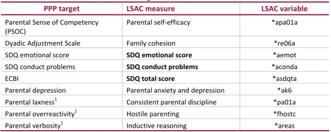
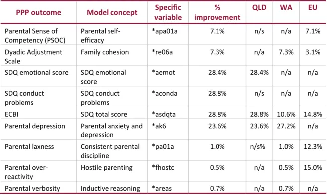
Table 6.4 : PPP target areas and LSAC variables ... 58

Table 6.5 : Impact of large scale Queensland PPP trial ... 58

Table 6.6 : Impact of large scale Western Australian PPP trial ... 59

Table 6.7 : Improvement in means scores of European PPP trial ... 60

(5)

Table 6.9 : PPP costs ($US) ... 61

Table 6.10 : Outcomes of PPP as delivered over 2004‐05 to 2007‐08 in Queensland... 61

Table 6.11 : ATP variables associated with the Reconnect Program ... 66

Table 6.12 : Estimate of effect size — young person’s perception of their ability to manage family conflict before Reconnect and now... 67

Table 6.13 : Estimate of effect size — young person’s perception of their family’s ability to manage family conflict before Reconnect and now ... 68

Table 6.14 : Outcomes of the Reconnect Program, as delivered over 2004‐05 to 2008‐09... 69

Table 6.15 : The value of PFF... 69

Table 7.1 : Summary of costs and benefits of modelled interventions ... 72

Table B.1 : Antisocial behaviour ... 88

Table B.2 : Anxiety and depression ... 88

Table B.3 : Smoking ... 89

Table B.4 : Alcohol... 89

Table B.5 : Illicit drug use ... 89

Table B.6 : Productivity ... 90

Table B.7 : Overweight/obesity... 90

Table C.1 : Obesity B1 (ahs23c2) ... 91

Table C.2 : Obesity B2 (bcbmi) ... 92

Table C.3 : Obesity B3 (ccbmi)... 92

Table C.4 : Obesity K2 (dcbmi) ... 93

Table C.5 : Obesity K3 (ecbmi)... 93

Table C.6 : Productivity B1 (awlrnoi) ... 94

Table C.7 : Productivity B2 (bwlrnoi)... 94

Table C.8 : Productivity B3 (cwlrnoi) ... 95

Table C.9 : Productivity K2 (dwlrnoi)... 95

Table C.10 : Productivity K3 (ewlrnoi) ... 96

Table C.11 : Anxiety and depression B1 (apedsgc)... 96

Table C.12 : Anxiety and depression B2 (bpedsef)... 97

Table C.13 : Anxiety and depression B3 (cpedsef) ... 97

Table C.14 : Anxiety and depression K2 (daemot) ... 98

Table C.15 : Anxiety and depression K3 (eaemot) ... 98

Table C.16 : Antisocial B1 (apedsgc)... 99

Table C.17 : Antisocial B2 (babitp) ... 99

(6)

Table C.19 : Antisocial K2 (daconda) ... 100

Table C.20 : Antisocial K3 (eaconda) ... 101

Table C.21 : Addictions B1 (apedsgc) ... 101

Table C.22 : Addictions B2 (babitp) ... 102

Table C.23 : Addictions B3 (casdqta) ... 102

Table C.24 : Addictions K2 (dasdqta)... 103

Table C.25 : Addictions K3 (easdqta)... 103

Table D.1 : Standard LSAC variables... 104

Table D.2 : Combinations of LSAC variables... 106

Illustrative distribution of categorical variables... 109

Table G.1 : Underengagement predictor variables... 118

Table G.2 : Completion of high school(a)(b) ... 118

Table G.3 : Completion of high school (only) v University degree(a)(b) ... 119

Table G.4 : Body mass index at 23‐24 years(a)(b)... 120

Table G.5 : ATP anxiety/depression 2002 crosstabulation ... 122

Table G.6 : Logistic regression results — child age 19‐20 years (year 2002)(a)(b) ... 122

Table G.7 : Logistic regression results — child age 19‐20 years (year 2002)(a)(b) ... 124

Table I.1 : Obesity prevalence rates and estimated obese people (number) in 2010 ... 136

Table I.2 : Anxiety and depression prevalence rates and estimated people with anxiety and depression (number) in 2010 ... 136

Table I.3 : Smoking prevalence rates and estimated current daily smokers in 2010... 137

Table I.4 : Prevalence rates for tobacco‐caused diseases and conditions(a)... 138

Table I.5 : Prevalence rates ‐ drinking at risky‐high risk(a) levels of long term health harm and estimated risky‐high risk drinkers in 2010... 138

Table I.6 : Prevalence rates for recent use(a) of illicit drugs and estimated recent users in 2010139 Table I.7 : Offender age‐gender prevalence profile and estimated offenders in 2008‐09 ... 139

Table I.8 : Prisoner age‐gender prevalence rates and estimated prisoners in 2009 ... 140

Table I.9 : Annual per‐person costs of obesity ‐ males (in 2010 dollars) ... 140

Table I.10 : Annual per‐person costs of obesity ‐ females (in 2010 dollars) ... 141

Table I.11 : Annual per‐person costs of anxiety and depression ‐ males (in 2010 dollars)... 142

Table I.12 : Annual per‐person costs of anxiety and depression ‐ females (in 2010 dollars) .. 142

Table I.13 : Annual per‐person costs of current daily smoking ‐ males (in 2010 dollars) ... 143

Table I.14 : Annual per‐person costs of current daily smoking ‐ females (in 2010 dollars)... 143

Table I.15 : Annual per‐person costs of alcohol abuse ‐ males (in 2010 dollars)... 144

(7)

Table I.17 : Annual per‐person costs of illicit drug abuse ‐ males (in 2010 dollars)... 145

Table I.18 : Annual per‐person costs of illicit drug abuse ‐ females (in 2010 dollars) ... 145

Table I.19 : Age‐gender employment in the general population ... 146

Table I.20 : Age‐gender average weekly earnings(a) for the general population ($) ... 146

Table I.21 : Annual costs of year 12 non‐completion ($ 2010) ... 147

Table I.22 : Annual costs of undergraduate degree non‐completion ($ 2010)... 147

Table I.23 : Age‐specific undergraduate non‐completion rates in 2007... 148

Table I.24 : Annual policing cost per offender ($) ... 149

Table I.25 : Annual court system cost per offender ($)... 149

Table I.26 : Annual prison system cost per prisoner ($)... 149

Table I.27 : Annual per‐person societal costs of crime for males ($)... 150

Table I.28 : Annual per‐person societal costs of crime for females ($)... 150

Table I.29 : Crime under‐reporting multipliers and derived probabilities ... 151

Table I.30 : Probabilities of court action on reported crimes ... 152

Table I.31 : Court finalisation outcome probabilities... 153

Table I.32 : Custodial sentence probabilities in guilty verdict court cases ... 153

Figures

Figure 2.1 : Approximate age of study cohorts and bridging the current information gap... 8

Figure 2.2 : Diagram of data map... 9

Figure 2.3 : Conceptual map for valuing costs of NFF... 10

Figure 2.4 : Incidence versus prevalence approach ... 10

Figure 2.5 : Cost effectiveness analysis model map... 17

Figure 2.6 : CEA model pathway for interventions ... 18

(8)

(9)

Acknowledgements

Access Economics would like to acknowledge with gratitude the expert knowledge and inputs

provided by members of the Expert Reference Group for this project.

Professor Ann Sanson

Department of Paediatrics, University of Melbourne, ARC/NHMRC Research Network

Coordinator, Australian Research Alliance for Children and Youth

Brian Babington

Chief Executive Officer, Families Australia

Carol Ey

Branch Manager, Research and Analysis Branch, Department of Families, Housing, Community

Services and Indigenous Affairs

Dr Lance Emerson

Chief Executive Officer, Australian Research Alliance for Children and Youth (ARACY)

Dr Marian Esler

Section Manager, Research Section, Family and Child Support Policy Branch, Department of

Families, Housing, Community Services and Indigenous Affairs

Dr Matthew Gray

Deputy Director, Australian Institute of Family Studies

Megan Shipley

Research Section, Family and Child Support Policy Branch, Department of Families, Housing,

Community Services and Indigenous Affairs

Paula Mance

Research Projects and Publications Section, Department of Families, Housing, Community

Services and Indigenous Affairs

Rachel Henry

Research Section, Family and Child Support Policy Branch, Department of Families, Housing,

Community Services and Indigenous Affairs

Professor Stephen Zubrick

Co‐Director for Developmental Health, Curtin University of Technology

Access Economics would like to acknowledge in particular the staff of the Australian Institute

of Family Studies (AIFS), who analysed the Australian Temperament Project (ATP) data and

modelled those regressions. Apart from Dr Gray, particular thanks go to Dr Ben Edwards and

(10)

Glossary

ABS Australian Bureau of Statistics

AE‐DEM Access Economics Demographic Model

AEM Access Economics Macroeconomics Model

AIFS Australian Institute of Family Studies

AIHW Australian Institute of Health and Welfare

AWE average weekly earnings

ATP Australian Temperament Project

B1, B2, B3 Baby cohort, waves 1, 2 and 3 in LSAC

BOD burden of disease

CALD Culturally and Linguistically Diverse

CBA cost benefit analysis

CEA cost effectiveness analysis

CFC Communities for Children

DALY disability adjusted life year

DCBA disease cost‐burden analysis

DEEWR Department of Education, Employment and Workplace Relations

DOFD Department of Finance and Deregulation

DSM Diagnostic and Statistical Manual

DSP Disability Support Pension

DWL deadweight loss

FAHCSIA Australian Government Department of Families, Housing, Community

Services and Indigenous Affairs

FF family functioning

FRS family relationship services

GP general practitioner

HILDA Household Income and Labour Dynamics in Australia

International Classification of Diseases (10th revision)

ICD‐10

K1, K2, K3 Kindy cohort, waves 1, 2 and 3 in LSAC

LSAC Longitudinal Study of Australian Children

LSAY Longitudinal Study of Australian Youth

NHS National Health Survey

NDHS National Drug Strategy Household Survey

(11)

NSA Newstart Allowance

NFF negative family functioning

MBS Medicare Benefits Schedule

OLS Ordinary Least Squares

PBS Pharmaceutical Benefits Scheme

PC Productivity Commission

PFF positive family functioning

PPP Postive Parenting Program

PS Parenting Scale

PSOC Parental Sense of Competency

PUP Parents under Pressure

QOL quality of life

REACH Responding Early Assisting Children

SCRGSP Steering Committee for the Review of Government Service Provision

SDAC Survey of Disability, Ageing and Carers (ABS)

SDQ Strengths and Difficulties Questionnaire

SES socioeconomic status

SFCS Stronger Families and Communities Strategy

TILA Transition to Independent Living Allowance

VSLY value of a statistical life year

WHO World Health Organization

W1,2,3 waves 1,2,3 of LSAC

YLD year(s) of healthy life lost due to disability

(12)

(13)

Executive

Summary

Access Economics was commissioned by the Australian Government Department of Families,

Housing, Community Services and Indigenous Affairs (FaHCSIA) to quantify, in economic terms,

the value of ‘goods and services’ provided by positive family functioning (PFF) and to conduct a

cost benefit analysis (CBA) to establish the returns to government and society for investments

made in supporting family functioning (FF). This report follows a scoping study, also conducted

by Access Economics, to establish the methodology for the project. The scoping study explains

the equivalence of measuring the value of PFF as the costs of negative family functioning

(NFF). This study was overseen by a panel of experts.

Methods

FF is defined through a variety of domains – emotional, governance, cognitive, physical, intra‐

familial and social (Table 2.1). Literature review revealed three broad areas of outcomes

associated with FF.

■

Health outcomes were observed through the occurrence of anxiety and depression,

obesity and substance abuse (smoking, alcohol and drug abuse) later in life. These are

associated with health expenditures, productivity losses (through lower workforce

participation and premature death), other financial costs, and loss of quality of life (QoL)

(measured in disability adjusted life years or DALYs).

■

Productivity outcomes were reflected in secondary and tertiary educational

achievement completion, flowing on to impact lifetime earnings.

■

Social outcomes were primarily measured through negative manifestations – antisocial

behaviour such as delinquency and crime, resulting in criminal justice system costs.

Two longitudinal studies — the Longitudinal study of Australian Children (LSAC) aged up to 9

years and the Australian Temperament Project (ATP) for older children were selected to

analyse the relationship between FF and child outcomes. Regression analysis was conducted

to establish relationships between ‘transition’ health, productivity and social outcome

variables in LSAC and FF variables. The latter were selected on the basis of literature evidence,

after controlling for other factors such as socioeconomic status (SES). Transition variables

were carefully selected to match similar or identical ATP variables. Further regression analysis

was undertaken using the transition variables, together with ATP FF and control independent

variables, to establish relationships with ATP ‘interim’ health, productivity and social outcomes

in early adulthood. The interim outcomes were then used to predict lifetime health,

productivity and social costs, based on an extensive costing process utilising multiple data

sources (Chapter 5).

Findings

The net present value (NPV) of benefits from intervening in childhood and adolescence to

prevent poor outcomes later in life are substantial, despite the fact that such intervention

incurs costs today but discounted benefits are realised a long time into the future.

In total, the potential NPV of benefits to be realised is in the order of $5.4 billion per

annum in 2010 dollars. This can be considered the cost of NFF currently, or the value of

PFF gains possible. Over half these gains (53% or $2.9 billion) are productivity gains,

with a further 22% ($1.2 billion) of the benefits deriving from savings from fewer

(14)

addictions. Fewer cases of anxiety and depression would save $0.6 billion (11%), while

lower rates of criminality and antisocial behaviour would accrue $0.5 billion (10%). A

reduction in obesity would save $0.3 billion per annum (5% of the total) ‐ Figure i. Figure i: Value of PFF by benefit type, 2010 (total $5.4 billion), $bn and % total 261 , 5% 2,882 , 53% 581 , 11% 547 , 10% 1,176 , 22%

Obesity Productivity Anxiety and depression Anti‐social Addictions

Source: Access Economics calculations. Note: Shares may not sum to 100% due to rounding.

is has focused on three interventions selected on ba

■

efit:cost ratio

tio

benefit:cost ratio for this return on investment.

Costs and benefits are summarised in Table ii.

There are also marked social and economic benefits if cost effective prevention programs can

be identified and implemented. This analys the ses of a range of criteria (section 2.6)

The Communities for Children program, targeting pre‐school and primary school aged

children, is one of the major Australian Government investments in families. The

program improves outcomes in various FF areas including hostile parenting, parenting

self‐efficacy, parent mental health, quality of the home learning environment, parental

relationship conflict, child total emotional and behavioural problems, childhood

overweight, receptive vocabulary achievement and verbal ability. The ben for this program was estimated as 4.8:1, a 377% return on investment.

■

The Positive Parenting Program is one of the best evaluated FF programs for younger

children. The program improves FF outcomes in parental sense of competency, the

dyadic adjustment scale, the Strengths and Difficulties Questionnaire (SDQ) emotional

and conduct scales, the Eyberg Child Behaviour Intensity score, parental depression,

parental laxness, parental over‐reactivity, and parental verbosity. The benefit:cost ra for this program was estimated as 13.8:1, a substantial 1,283% return on investment.

■

The Reconnect program targets an older cohort of children and was found to improve

outcomes in school bonding and conflictual relationships, with proxied effect sizes

estimated for attachment to parents and harsh parenting. The

(15)

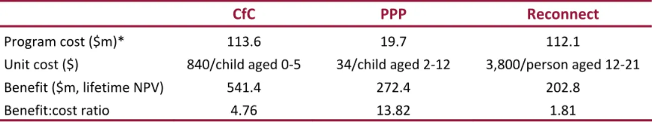
Table ii: Summary of costs and benefits of modelled interventions

CfC PPP Reconnect

Program cost ($m)* 113.6 19.7 112.1

Unit cost ($) 840/child aged 0‐5 34/child aged 2‐12 3,800/person aged 12‐21

Benefit ($m, lifetime NPV) 541.4 272.4 202.8

Benefit:cost ratio 4.76 13.82 1.81

Source: Access Economics calculations. * Costs estimated over 2004‐05 to 2007‐08 except for Reconnect which extends to 2008‐09.

Many of the family ‘inputs’ incorporated in the analysis were found to be statistically

significant explanators of child outcomes with the relationship consistent with that predicted

by the literature.

■

Obesity was explained by key drivers such as previous obesity, parental obesity, lack of

child persistence, and parent‐child conflict.

■

Anxiety and depression were dependent on previous emotional problems, difficult

temperament, lower socioeconomic status (SES), harsh discipline, parental

anxiety/depression, alienation from parents and lack of child persistence.

■

Smoking in young adulthood (19‐20 years) was determined by previous smoking in

adolescence, parental permission to smoke at home and a conflictual parent‐teenager

relationship. Alcohol abuse (binge drinking) in young adulthood was dependent on teen

bingeing, lack of parental monitoring, father drinking and initiating drinking at an older

age (over 15 compared to 14 or younger). Illicit drug use in 23‐24 year olds was

dependent on the child’s temperament, lack of parental monitoring, and mother

smoking.

■

Predisposition to smoking, alcohol abuse and illicit drug use was established in early

years by parental smoking, temperament, harsh and/or inconsistent discipline, poor

nce,

king and low

SES, along with parental anxiety/depression and the child’s temperament.

te these

findings internationally as well as continue to enhance the evidence base in Australia. Access Economics

family cohesion and parental anxiety depression.

■

Productivity was driven by previous learning outcomes, consistent discipline,

temperament, socioeconomic status, parent education and, in adolescence, persiste relationship quality/warmth, parental monitoring and a positive attitude to school.

■

Antisocial behaviour and outcomes were determined by child lack of persistence,

previous social/conduct problems and, importantly, were largely influenced by early life

FF variables such as poor family cohesion, harsh discipline, parental smo

The greatest value in this project has been primarily to showcase how a broad, quantitative

approach to social policy evaluation can work. With better quality data in the future, there is

scope to refine and continue to develop the modelling and elaborate on findings further. The

scope of this project has been both ambitious and challenging but, we believe, the methods

developed and many findings and insights are of global significance. The novelty of the

(16)

(17)

1

Introduction

Access Economics was commissioned by the Australian Government Department of Families,

Housing, Community Services and Indigenous Affairs (FaHCSIA) to quantify, in economic terms,

the value of ‘goods and services’ provided by positive family functioning (PFF) and to conduct a

cost benefit analysis (CBA) and/or cost effectiveness analysis (CEA) to establish the returns to

government and society for investments made in supporting family functioning.

This report follows a scoping study, also conducted by Access Economics. The scoping study in

2009 determined:

■

the feasibility of quantifying, in economic terms, the value of ‘goods and services’

provided by PFF;

■

a method for measuring the benefits of PFF; and

■

a method to conduct CBA and CEA of interventions to improve FF.

The methods developed in the scoping study form the basis for the analysis in this report. The

scoping study explains the equivalence of measuring the value of PFF as the costs of negative

family functioning (NFF).

Both the scoping study and this full study were overseen by a panel of experts, as listed in the

acknowledgements section of each report. In addition, this study was undertaken with

assistance from the Australian Institute of Family Studies (AIFS), which analysed the Australian

Temperament Project (ATP) data.

The structure of this report is as follows.

■

The methodology is explained in chapter 2.

■

The findings from the investigation of the Longitudinal Survey of Australian Children

f the ATP are detailed in chapter 4.

nd the CEA results are explained.

etailed information is provided in the Appendices in relation to the methods, LSAC and

ATP investigations, and the costing model.

(LSAC) are outlined in chapter 3.

■

The findings from the investigation o

■

The costing model is described in 5.

■

In chapter 6, the interventions analysed a

■

Conclusions are elaborated in chapter 7.

(18)

2

Methodological

overview

2.1

Definition

of

family

functioning

and

the

outcomes

of

interest

The focus of the scoping study was on the outcomes of family functioning for the child,

without pursuing any family ‘ideal’ or promoting any specific type of family structure. Children

are not able to explicitly control their family environment and they are often viewed as the

main victims of NFF.

The scoping study identified that while no simple definition of PFF exists, consistent themes (or

‘domains’) of FF emerged from the literature. These were developed and agreed, in

consultation with the Expert Reference Group for the scoping study and with FaHCSIA. These

domains provide an overarching definition of the FF environment. A summary is provided

below.

Family functioning (FF) – positive and negative – is defined through a variety of emotional attributes, family governance frameworks, cognitive engagement and development characteristics, physical health habits, intra‐familial relationships and social connectedness. PFF is characterised by emotional closeness, warmth, support and security; well‐communicated and consistently applied age‐ appropriate expectations; stimulating and educational interactions; the cultivation and modelling of physical health promotion strategies; high quality relationships between all family members; and involvement of family members in community activities.

The domains of FF are not mutually exclusive, but interact, complement each other and co‐

exist.

Table 2.1: Characteristics of family functioning domains Domain Characteristics / Proxies

Emotional Closeness of parent‐child relationships, warmth, responsiveness,

sensitivity, perceived parental and family support as well as healthy

open communication, and security/safety.

Governance Establishment of age‐appropriate rules, expectations and consistency

Engagement and cognitive

development

Reading and verbal engagement, quality time fostering the development of educational, language and interaction skills. Physical health

Healthy/unhealthy physical activities or environments as well as access – including in‐utero – to specific products (e.g. fruit and vegetables, cigarettes and alcohol).

Intra‐familial relationships (dyadic family relationships)

Quality of relationships between all members of the family. For example sibling rivalries, parent‐child relationships as well as the health of the parents’ relationship.

Social connectivity Involvement of parents and children in activities outside of the family

unit (e.g. school, community service, volunteer work). Also includes relationships with extended family and work/life balance.

(19)

The literature review for the scoping study revealed three broad areas of outcomes associated

with FF.

■

Health outcomes were mostly observed through the occurrence of mental illnesses such

as anxiety and depression later in life, but also included eating disorders, health

behaviours (e.g. unsafe sex, physical inactivity, overweight and obesity) and substance

abuse (e.g. smoking, alcohol and drug abuse), with the consequent physical impacts of

these risk factors on morbidity and mortality outcomes.

■

Productivity outcomes were reflected in rates of labour force participation,

employment and hourly wage rates, with a number of intermediate measures reported

in the literature, such as reduced levels of literacy and numeracy and other measures of

educational achievement.

■

Social outcomes were measured primarily through their negative manifestations – involvement in antisocial behaviour such as delinquency, and the probability of criminal

behaviour during youth and later in life. In contrast it was harder to quantitatively

associate PFF with positive manifestations such as the quality of inter‐personal

relationships and future community contributions.

The criteria used to select the specific outcomes for analysis in this report were:

■

each outcome domain was covered (health, productivity and social);

■

outcomes were associated with high economic and social costs, including burden of

were able to be measured by the data sets used as the basis for analysis

(see below).

this

ree);

sion, obesity, smoking, drinking, illicit drug use); and

ile

aic of

thy study timeframes. For example, intermediate outcomes

y and literacy cannot easily be converted into specific types of jobs and streams.

investigated but the LSAY did not

disease (BoD), based on prevalence and/or existing studies of costs and BoD;

■

the outcomes

In report, the correlation between FF is thus examined for the following outcomes:

■

productivity (school completion and completion of an undergraduate university deg

■

health (anxiety and/or depres

■

social (antisocial behaviour).

Wh the literature provided valuable insights into potential linkages between FF and child

outcomes, the following cautions apply.

■

Many of the concepts are difficult to capture and measure and there is a mos different and overlapping instruments and metrics.

■

Statistical techniques can be used to determine correlation rather than causation.

■

While measures of intermediate outcomes are available, it is difficult to convert these to

final outcomes without leng such as numerac

lifetime earnings

2.2

Data

review

Two longitudinal studies — the Longitudinal study of Australian Children (LSAC) and the

Australian Temperament Project (ATP) were selected to analyse the correlation between FF

and child outcomes. The Longitudinal Survey of Australian Youth (LSAY) and the Household,

(20)

col t information on FF variables and HILDA is limited to relationships between the family

nment and parent’s participation in the labour force.

LSAC has the advantage of containing a breadth of data, valuable for testing

confo lec enviro

■

unding factors. However, a disadvantage is the relatively short timeframe of data

years. However, measures

gers

du ,

however, eptual consistencies in measurement of FF between the two data sets.

collection as the eldest participants from the child cohorts are currently 10‐11 years of

age.

■

ATP is currently the only study in Australia that allows the determination of long term

impacts of FF on health, economic and social outcomes as the most recent data for

participants in this study were collected at the age of 23‐24

of FF and parenting have only been recorded since the participants were in their early

teens, with no measures during infancy or early childhood.

Variables from the ATP and LSAC within each of FF domains were mapped to the specific

outcomes selected for analysis so that the likelihood of one of the events of interest occurring

could be established across different age groups (Figure 2.1) and linked with outcomes. The

ability to join information from LSAC and ATP is limited by slightly different methods in each

data set of measuring FF and differences in the generations (ATP children were teena ring the 1990s, whereas LSAC children are growing up during the new century). There are

conc

Figure 2.1: Approximate age of study cohorts and bridging the current information gap

LSAC (1)

LSAC (2) Current Age Cohort Data Gap

ATP

0 1 2 3 4 5 6 7 8 9 10 11 12 13 14 15 16 17 18 19 20 21 22 23 24 25 26 27 28 29 30

Approximate Age of Cohort in 2009

LSAC (1) is the Birth cohort and LSAC (2) is the Kindy cohort.

Ideally, one or two more waves of information from the LSAC is required to successfully bridge

the gap in ages between the two studies, to enable mapping outcomes for children aged

analys

■

observations in the oldest groups

i.e. the third wave of the Kindy cohort in LSAC. Early and mid‐period FF and control

P

ep analys

9 years to those aged 13 years. This approach is considered acceptable, given the alternative is

to wait some years for additional study waves to be completed.

Figure 2.2 shows how LSAC provides the dependent (end‐period ‘transition’) variables and

independent (early and mid‐period family functioning and control) variables in regression

is of children aged up to 9 years.

End‐period transition variables are those that relate to

variables relate to observations in all the other age groups (the first and second wave

observations and the third wave for the birth cohort).

AT data then provide the dependent (end‐period ‘interim outcome’) variables and

ind endent (early and mid‐period family functioning and control) variables in regression

(21)

■

ion completed, illicit drug use and body mass index were assessed at age

23‐24 years, while other variables (completing year 12, smoking, binge drinking,

n be modelled by ‘shocking’ the LSAC variables, while

adolescent interventions1_can _by_{‘shocking’}_the_ATP_variables._{‘Shocking’}_the

model refers to changing inpu simulating the effects of

an intervention, and then observing the consequent change in model outputs (health,

End‐period interim outcome variables are those that relate to observations in the oldest

groups of ATP relevant to the cost data and the circumstance. For example, highest

level of educat

anxiety/depression, and anti‐social behaviour) were assessed at adulthood (18‐19

years). Early and mid‐period FF and control variables relate to younger age

observations.

The interim outcomes can then be used to predict, in an Excel model, lifetime health costs,

lifetime productivity losses, social costs of crime and disability adjusted life years (DALYs). The

impact of childhood programs ca

be modelled

t parameters from one level to another, productivity and social outcomes).

Figure 2.2: Diagram of data map

LSAC ‐ early and mid‐period

CfC, PPP shock FF variables

control variables (confounding) Regression analysis

LSAC ‐ end‐period ATP ‐ early and mid‐period

Transition variables FF variables shock Reconnect

control variables (confounding) Regression analysis ATP ‐ end‐period

Interim outcomes Excel model Lieftime health costs Productivity (lifetime earnings) Social (lifetime costs of crime) DALYs

In laymen’s terms, LSAC was used to establish the impact of FF on children up to the age of

9 years, at which age transitional outcomes from childhood were spliced into the ATP analysis

by matching this set of transitional outcomes across the two datasets. Health, productivity

ng adequate data to establish

hip between family functioning and outcomes, collaborative relationships were

chers and FaHCSIA data specialists. Both were important

participants in the project. Furthermore, AIFS currently manages the ATP data set and access

and social interim outcomes in early adulthood thus depended on FF during adolescence as

well as the transitional outcomes from childhood. From the interim outcomes in early

adulthood, lifetime cost impacts were predicted using a variety of other datasets.

Given the identification of the ATP and LSAC databases as providi the relations

established with AIFS resear

arrangements require that AIFS undertake any in depth analysis.

1

The Communities for Children (CfC) and Positive Parenting Program (PPP) were selected for younger children, while the Reconnect program was selected for adolescents (see Section 2.6).

(22)

2.3

Literature

review

Evidence from the literature was used to edify the selection of family functioning inputs from

es. The findings are briefly

outlined in chapter 3, and chapter 4, and evidence is summarised in Appendix A and Appendix

2.4

Concepts

a

the ATP and LSAC that would be likely to be correlated with outcom B.

nd

data

underlying

lifetime

costing

Costs were attached to each outcome as depicted in Figure 2.3.

Figure 2.3: Conceptual map for valuing costs of NFF

Emotional Health Health system expenditures Governance Productivity losses

Cognitive Productivity Criminality costs Physical Social/criminality DWLs

Intra‐familial Other financial impacts Social Burden of disease

Source: Access Economics. Blue – health impacts. Red – productivity impacts. Green – Social/criminality impacts.

An incidence or ‘life aetiology of lagged

outcomes – i.e. ‘lifetime’ costs (hazard model). An incidence approach is distinguished from a

time’ costing approach was adopted in line with the prevalence approach in Figure 2.4.

Figure 2.4: Incidence versus prevalence approach

2000

2009

2018

A*

A

B*

B

B**

C

C*

Incidence

costs

(2009)

=

C

+

present

value

of

C*

Prevalence

costs

(2009)

=

A

+

B

+

C

The lif diseas

■

Cost Data Collection

(Department of Health and Ageing), the Pharmaceutical Benefits Scheme (PBS), the Note: The years are illustrative and do not relate to this analysis.

etime costs associated with each outcome include the standard cost categories for

e cost burden analysis from the health economics literature:

Direct health costs – estimated with cost data sourced primarily from the Australian

(23)

Medicare Benefits Schedule (MBS) and epidemiological data sourced from the Australian

Bureau of Statistics (ABS) National Health Survey (NHS), AIHW and other specific

epidemiological studies reported in the peer reviewed literature.

re

(unpaid care provided by family and friends), health aids and appliances, deadweight

sources of these estimates are previous studies by Access Economics, and the ABS

and Carers (SDAC) (ABS, 2004), and Lattimore et al (1997).

is s

the co lected for analysis. The net

se

■

nt a direct input into the cost benefit analysis.

analyses) change as a result of the intervention

pact of a 'shock' to consistent

■

Costs of crime – estimated with data primarily from the Steering Committee for the

Review of Government Service Provision (SCRGSP) Report on Government Services, and

reports from the Australian Institute of Criminology and ABS. .

■

Productivity costs – are estimated using the human capital approach and reflect

reduced labour force participation and absenteeism due to the outcomes selected.

Parameters and labour force data were drawn primarily from the ABS and reports by the

Productivity Commission (PC), as well as peer reviewed literature.

■

Burden of disease (BoD) – was estimated using DALYs and determined using the same

disability weights and methodology used by the AIHW (Begg et al, 2007). Monetary

values were estimated for the BoD using the value of a statistical life year from DOFD

(2009).

■

Other financial costs – include costs associated with the provision of informal ca losses (DWLs) (efficiency losses which arise due to transfer payments). The main Survey of Disability, Ageing

Further detail on costing methods, cost categories and data sources is provided in Appendix I.

2.5

Model

construction

Th ection provides an outline of the model developed to investigate the benefits of PFF and

sts and benefits of the three family functioning programs se

benefits for each program were derived under a scenario with the intervention compared to a

‘ba case’ without the intervention.

The costs for the CfC program, PPP and Reconnect programs are reported in chapter 6

and represe

■

The benefits are based on the extent to which each intervention improves FF and

reduces its associated costs. The effectiveness of each intervention is reported in

chapter 6 while the associated costs (health, productivity and social) are detailed in

chapter 5.

The underlying principle of the model (developed in Microsoft Excel 2007) is that outcomes

(dependent variables in the regression

affecting early and mid‐period family functioning (independent) variables in the regression.

The size of the intervention is a direct function of the effectiveness of the program on

impacted functioning variables (chapter 6) and the size of the coefficients derived in the

regressions (Appendix C and Appendix G).

A simple example illustrates the model construction using the im

discipline on anxiety in children aged 4‐5 (so the analysis starts with the B3 cohort of this age –

incidentally the same age as the K1 cohort). The ‘shock’ in this example was derived from PPP

improvements in ‘parental laxness’ and mapped directly to parental consistent discipline as

(24)

The 'shock' can be viewed as changing the input parameters (e.g. parental consistent

discipline) from one level to another, simulated by the effects of an intervention. Before the

shock, the multivariate regressions for anxiety are given below for age group 4‐5 (B3), 6‐7 (K2)

and 8

anxiet child, and discipline is towards that child).

‐9 (K3), respectively. In each case, i represents the observational child in the dataset (so

y is that of the

Where:

B3 = Cohort of children aged 4‐5 in the ("Baby") group B2 = Cohort of children aged 2‐3 in the ("Baby") group

= Beta coefficient for 'Anxiety' in group B2

= Beta coefficient for 'Consistent discipline' in group B3 = Regression error term

Where:

K2 = Cohort of children aged 6‐7 in the ("Kindergarten") group B3 = Cohort of children aged 4‐5 in the ("Baby") group

= Beta coefficient for 'Consistent discipline' in group K2 = Regression error term

Where:

K3 = Cohort of children aged 8‐9 in the ("Kindergarten") group K2 = Cohort of children aged 6‐7 in the ("Kindergarten") group

= Beta coefficient for 'Anxiety' in group K2

= Beta coefficient for 'Consistent discipline' in group K3 = Regression error term

(25)

As a result of the intervention, the new level of childhood anxiety for children aged 4‐5

includes changes in parental consistent discipline. The change in parental consistent discipline

from the shock was calculated by multiplying the effectiveness of the program by the average

onsistent discipline value for children aged 4‐5.

c

Where:

= New 'Anxiety' value after intervention

= (mean consistent discipline x effectiveness of

program)

= Beta coefficient for 'Consistent discipline' in group B3 B3 = Cohort of children aged 4‐5 in the ("Baby") group

B2 = Cohort of children aged 2‐3 in the ("Baby") group = Regression error term

As a result of the shock, the consequent change in the model output (Anxiety') is given by a

ercentage change. p Where:

= Percentage change in 'Anxiety' = New 'Anxiety' value after intervention = Baseline 'Anxiety' value

B3 = Cohort of children aged 4‐5 in the ("Baby") group B2 = Cohort of children aged 2‐3 in the ("Baby") group

Consequently, the direct percentage change in anxiety levels for children in the 4‐5 age group

is captured through to the next LSAC age group (6‐7 year group) through the use of the lagged

ependent variable changing by the intervention effectiveness.

(26)

Where:

= Percentage change in 'Anxiety' = New 'Anxiety' value after intervention

= Baseline 'Anxiety' mean value B3 = Cohort of children aged 4‐5 in the ("Baby") group B2 = Cohort of children aged 2‐3 in the ("Baby") group

Where:

= New 'Anxiety' value after intervention in the previous age group = New 'Anxiety' lagged dependent variable = as above

= Beta coefficient for 'Consistent discipline' in group B3 K2 = Cohort of children aged 6‐7 in the ("Kindergarten") group B3 = Cohort of children aged 4‐5 in the ("Baby") group

= Regression error term

Following this pattern, Anxiety’’K2,i and Anxiety’K3,i are similarly calculated. The change in the

final period of LSAC compared with the actual outcome is then included in the ATP multinomial

logit regression i.e. the new anxiety levels for K3 children aged 9 (the final regression in the

(27)

Where:

= New 'Anxiety' value in children aged 8‐9 in the ("Kindergarten") group = Base 'Anxiety' value in children aged 8‐9 in the ("Kindergarten") group

This effectively assumes that no change occurs in outcomes between the ages of 10 to 12. As

mentioned before, this approach is considered acceptable, given the alternative is to wait

some years for additional study waves to be completed.

The multinomial logit regression models were used to analyse the impact of an intervention on

the probability of each family functioning outcome for children aged 13‐23 years. Unlike the

multivariate linear regressions, the results presented in the logit regression represent the

probability of an outcome for a person with ‘average’ attributes. Like the LSAC multivariate

linear regressions, the interventions were modelled as a deviation from the mean of a

particular explanatory variable (e.g. anxiety). The baseline logistic regression is given below,

where e is a mathematical constant, i is again each child observed (in ATP this time), βs are

again coefficients, and

ε

s are again error terms. X is the sample mean.

After the percentage change from anxiety in the 8‐9 year old age group, the new logistic

regression is given, with changes to the lagged dependent variable.

In using the multinomial logit model, coefficient estimates are not directly interpretable so do

not provide the same type of information as coefficients from an Ordinary Least Squares (OLS)

model. A more natural way of interpreting results from a multinomial logit model is to

determine the impact on the probability of an outcome by changing the variables that would

be impacted by the intervention while holding all others constant. The impact of the

intervention on the probability can therefore be represented by:

The impact of the intervention was therefore measured as the difference between the

probability of an outcome for an average person with and without the intervention. As such,

the model projects the probabilistic change in the outcome as a result of the intervention and

(28)

between the scenario and the ‘base case’ (no intervention) can therefore be evaluated to

determine the intervention’s overall return on investment using a dollar value.

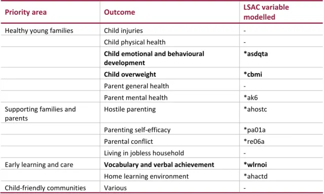
Table 2.2 summarises all the FF variables in the model for each intervention modelled

(i.e. found to be significant in the regression analysis reported later on). A conceptual map of

the model is provided in Figure 2.5.

Table 2.2: FF variables used for each intervention

CfC PPP Reconnect

Hostile parenting Hostile parenting Harsh parenting

Parenting self‐efficacy Parental self‐efficacy

Consistent parental discipline

Attachment to parents

Parental warmth*

Parental relationship conflict Family cohesion Conflictual relationships

Parent mental health Parental anxiety and depression

Child total emotional and behavioural

problems (SDQ)

SDQ total score, SDQ emotional score, SDQ conduct problems

Quality of the home learning

environment

Home learning environment*

Receptive vocabulary achievement

and verbal ability

Inductive reasoning School bonding (positive affect

towards school); Under‐engagement

(not in education or training and not

employed)*

Child overweight

Source: Access Economics (2010). Note: See Chapters 3, 4 and 6 for derivation. * These variables are in the Reconnect model but the effect size was estimated as zero.

(29)

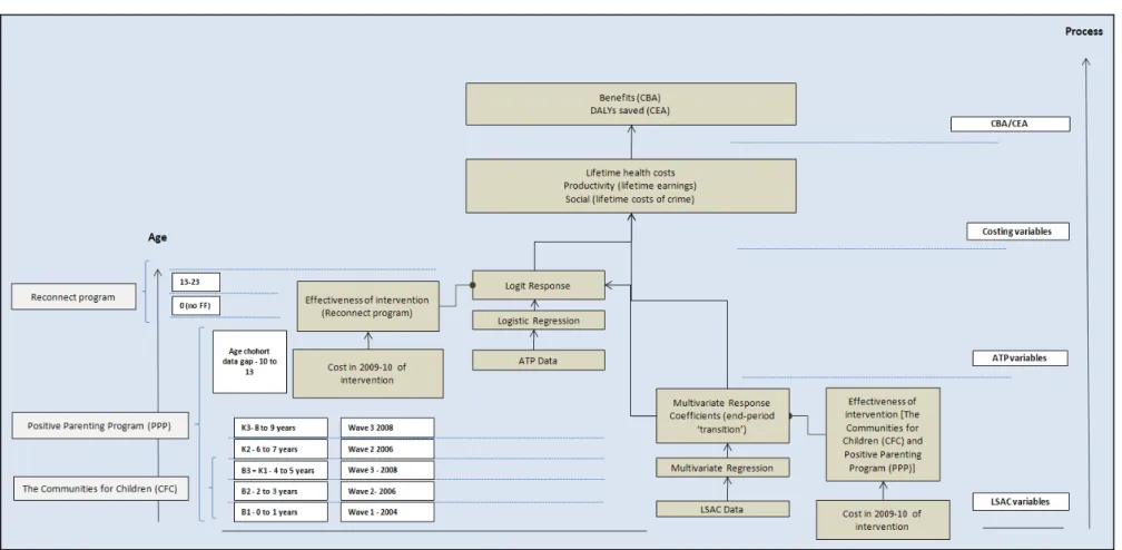
Figure 2.5: Cost effectiveness analysis model map

Source: Access Economics (2010)

(30)

2.6

Cost

benefit/cost

effectiveness

analysis

(CBA/CEA)

and

the

process

for

selecting

interventions

for

analysis

The concept of CEA modelling of FF interventions is outlined in Figure 2.6. All analyses

compare the outcomes for children with the interventions, against outcomes for children

without the intervention. The efficacy of a selected intervention in improving FF is derived

from previous evaluations of the programs. The Excel model is then used to explore how this

improvement in FF (the ‘shock’) reduces lifetime costs (in dollars and DALYs). These lifetime

benefits can then be compared with the intervention costs, in net present value (NPV) terms. Figure 2.6: CEA model pathway for interventions

Intervention

Improvement in family functioning in

Yr x (efficacy)

Reduces lifetime costs (NPV in Yr x, discounted

DALYs saved )

Cost in 09‐10$ Benefit in 09‐10$ CBA $:$ Benefit:Cost ratio

DALYs saved CEA $/DALY saved

As noted in Section 2.2, ‘shocking’ the model for CBA and CEA involves comparing what

happens in the absence of an intervention (the status quo), with what would happen if a

particular target population received an intervention. The intervention improves FF based on

evaluated effectiveness of the program, which in turn improves transition and/or interim

outcomes (based on the coefficients derived from the modelling). Better outcomes are

associated with lower costs, so the NPV of the benefits (lower costs of NFF) can then be

compared with the costs of the intervention. Benefits minus costs provide the ‘net benefit’ in

dollars, while benefits divided by costs provide the ‘benefit:cost ratio’.

The process of selecting appropriate FF interventions commenced in the scoping study, when a

preliminary assessment was undertaken of 12 types of interventions:

1. family assistance and income support payments;

2. family relationship services (FRS);

3. Stronger Families and Communities Strategy, including Communities for Children and

Invest to Grow;

4. Positive Parenting Program (PPP);

5. Early childhood education;

6. Peel Child Health Survey;

7. Responding Early Assisting Children (REACh);

8. Reconnect;

9. Youthlinx;

10. Transition to Independent Living Allowance (TILA);

11. SureStart; and

(31)

For this full study, criteria were established in the first Reference Group meeting for assessing

appropriate interventions for CEA. These four criteria were:

1. Model data: the LSAC and ATP datasets will be able to accommodate ‘shocks’ to the

intervention;

2. Target age: the interventions will target different age groups (e.g. pre‐school, primary

school, youth)

3. Reach: the interventions have ‘reach’ i.e. they effectively target relevant

(disadvantaged) groups; and

4. Efficacy data: adequate information is available from Australian (preferably) or

international sources in order to provide an indication of the efficacy of interventions.

A follow‐up meeting with Steve Zubrick identified three further criteria.

5. Specificity: Interventions specifically target family functioning, rather than indirectly

affect it (e.g. income supplementation can assist with FF, but is in essence a poverty

alleviation method).

6. Sustainability: Interventions are current, and likely to continue into the future.

7. Relevance: Interventions have strong connections to or relevance for FaHCSIA.

We also reviewed literature provided by the Reference Group – Karoly et al (2007) and Wise et

al (2005). The interventions selected from this process are summarised below.

2.6.2

Communities

for

children

(CfC)

CfC meets all criteria for the CEA.

1. Model data: LSAC FF data can be linked with CfC interventions.

2. Target age: CfC is targeted to pre‐school and primary school age children.

3. Reach: CfC targets all Australian population sub‐groups.

4. Efficacy data: CfC has been evaluated with efficacy outcomes that can be imputed to

the Excel model.

5. Specificity: CfC aims to improve family functioning and outcomes for children.

6. Sustainability: The CfC program has forward funding.

7. Relevance: CfC is a FaHCSIA program.

Conclusion: CfC is one of the major Australian Government investments in

families. It has already been shown to be efficacious, and the CEA evaluation can

also determine at what cost its effective outcomes are achieved.

2.6.3

Positive

Parenting

Program

PPP meets all criteria for the CEA.

1. Model data: LSAC FF data can be linked with PPP interventions.

2. Target age: PPP is targeted to pre‐school and primary school age children.

3. Reach: PPP targets all Australian population sub‐groups.

4. Efficacy data: PPP has been evaluated with efficacy outcomes that can be imputed to

(32)

5. Specificity: PPP aims to improve family functioning and outcomes for children.

6. Sustainability: The PPP program is successful and growing.

7. Relevance: PPP is a program relevant to FaHCSIA core business.

Conclusion: PPP is one of the best evaluated programs targeted at improving

family functioning and outcomes for younger children. While its efficacy is well‐

proven, there are fewer studies on its cost effectiveness and this CEA can also act

as a tool to test/triangulate the power of the model.

2.6.4

Reconnect

In the Scoping Study Reference Group and in the 13 January Reference Group meeting the

Reconnect program was identified as being a good candidate for CEA. Again it meets all

criteria for the CEA.

1. Model data: ATP FF data can be linked with Reconnect interventions.

2. Target age: Reconnect targets youth aged 12‐18 (who are homeless or at risk of

homelessness) and their families.

3. Reach: Reconnect targets all Australian population sub‐groups.2

4. Efficacy data: Reconnect has been evaluated with efficacy outcomes that can be

imputed to the Excel model (based on two longitudinal studies).

5. Specificity: Reconnect aims to improve family functioning and outcomes for high school

aged children.

6. Sustainability: The Reconnect program is funded into the future.

7. Relevance: Reconnect is a FaHCSIA program.

Conclusion: Reconnect provides a complementary intervention targeted at an the

older cohort of children, which has been evaluated as effective, but where

nothing is yet known regard cost effectiveness.

2

Indigenous youth comprised 9% of the respondents to the longitudinal survey that formed a key element of the 2003 evaluation by the Australian Government Department of Family and Community Services (FACS, 2003:34) and ‘No differences exist between entering and exiting clients in relation to country of birth or language background’ (FACS, 2003:35). Youth were represented from all jurisdictions, from both sexes and with varying levels of case

(33)

3

Findings

from

the

LSAC

data

investigation

LSAC consists of two cohorts ‘B’ (for Baby) and ‘K’ (for Kindergarten). Each of these cohorts

has three sets of time data ‐‘waves’ of survey data taken at two yearly intervals. Information is

collected through self‐reporting and also observational measures (such as parent‐child

interactions). Child outcomes are measured as: behavioural and emotional adjustment;

language and cognitive development; and social competence.

LSAC contains specific research questions. One question focuses particularly on the impacts of

family relationships, composition and dynamics on child outcomes, and changes to these over

time. The question includes the analysis of:

■

the size and make‐up of family;

■

the involvement of extended family;

■

roles of family members;

■

character of parental relationships and level of conflict in the family;

ies, particularly in times of stress.

to represent

se

Appendix D provides a detailed description of each individual variable.

Cases

■

lationships between children and parents. In

■

parenting practices;

■

child’s temperament;

■

impact of family break‐up and re‐formation; and

■

family coping strateg

3.1

LSAC

variables

Evidence from the literature was used to edify the selection of family functioning inputs from

the ATP and LSAC that would be likely to be correlated with outcomes. The evidence is in Appendix B. In most cases, the choice of relevant LSAC variables

summarised

the general literature categories in the model is fairly straightforward. �