Eliminating Inefficient Cross-Layer Interactions in Wireless Networking

(1)

in Wireless Networking

Von der Fakultät für Mathematik, Informatik und Naturwissenschaften der Rheinisch-Westfälischen Technischen Hochschule Aachen

zur Erlangung des akademischen Grades eines Doktors der Naturwissenschaften genehmigte Dissertation

Vorgelegt von Diplom-Informatiker

Reiner Eric Ludwig aus Bishop, California (USA)

Berichter:

Prof. Dr. rer. nat. Otto Spaniol

Prof. Randy H. Katz Ph.D. (University of California at Berkeley) Tag der mündlichen Prüfung: 04.04.2000

(2)

the past five years.

I would like to thank Prof. O. Spaniol and Prof. R. H. Katz for their advice.

Many thanks to Almudena Konrad, Kimberly Oden, Bela Rathonyi, and Keith Sklower who contributed to the development of the measurement tools and the collection of many hours of traces.

This work greatly benefited from disscussions with Badri Badrinath, Hari Balakrishnan, Stephan Bauke, Jean Bolot, Mikael Degermark, David Eckhardt, Andreas Fasbender, Sally Floyd, Tom Henderson, Anthony Joseph, Roger Kalden, Phil Karn, Markku Kojo, Michael Meyer, Venkata Padmanabhan, and Vern Paxson.

Last but not least I want to thank Norbert Niebert, Frank Reichert, Olle Viktorsson, and Fiona Williams for supporting my work within Ericsson Research.

(3)

Introduction and Outline

The Internet has evolved into the communication medium of the future. It will not be long before virtually all people-to-people, people-to-machine, and machine-to-machine communi-cation are carried end-to-end in Internet Protocol (IP) [RFC791], [RFC2460] packets. The recent tremendous growth of the Internet in terms of connected hosts is only matched by the similar growth rate of cellular telephone subscribers. While most hosts on today’s Internet are still wired, the next big wave of hosts has yet to hit the Internet. We believe that the predomi-nant Internet access of the future will be wireless. Not only every cellular phone, but the major-ity of general communication devices will have: (1) an IP protocol stack and (2) a wireless net-work interface.

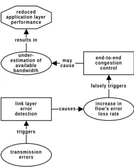
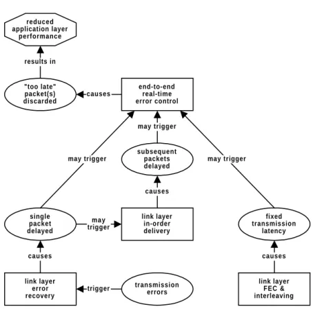
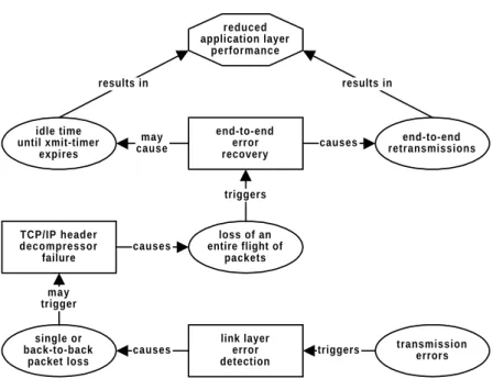
Wireless networking and more specifically, the problems related to protocol performance of “IP over Wireless”, are high priority research topics in both academia and industry. Yet, a num-ber of difficult problems remain unsolved. The root of these lies in inefficient cross-layer inter-actions, caused by events occurring at the link layer that affect the performance of end-to-end error and congestion control schemes (see Figure 1-1). Those events are packet losses due to transmission error and increased packet transmission delays caused by link layer error control. The goal of this dissertation is to study inefficient cross-layer interactions in wireless net-working and to develop and evaluate a solution that eliminates these inefficiencies.

End-to-End Error Control End-to-End

Congestion Control

Link Layer Error Control in Wireless Networks

Cross-Layer Interactions

(8)

Internet traffic today is still largely generated by applications that use the Transmission Control

Protocol (TCP) [RFC793] as the underlying communications protocol. The most popular

Internet applications, namely World Wide Web (WWW), e-mail, and file transfer, all rely on TCP. In the Internet backbone studied in [TMW97], the authors find that TCP averages about 80 percent of the flows. Related traffic analysis studies find similar numbers. This motivates why TCP has been the focus when it comes to studying inefficient cross-layer interactions in wireless networking.

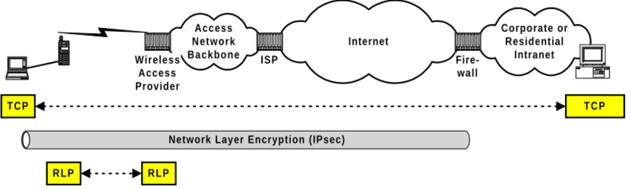
The solution we develop in this dissertation is, however, not “TCP-specific”, but is indepen-dent from any specific protocol. Nevertheless, to demonstrate the feasibility of our approach, most of our measurements, analysis, and implementation work is based on TCP. Our solution comprises new end-to-end and link layer mechanisms that make the protocol implementations on those layers more “intelligent” and robust. For flows that are loss responsive and fully-reli-able, in particular those based on TCP, our solution eliminates all known inefficient cross-layer interactions. It provides optimal end-to-end performance over a wide range of conditions of the wireless link while efficiently utilizing radio resources. Beyond solving the problems for such flows, our solution provides a framework that accommodates loss responsive real-time flows, e.g., semi-reliable, or error-resilient flows.

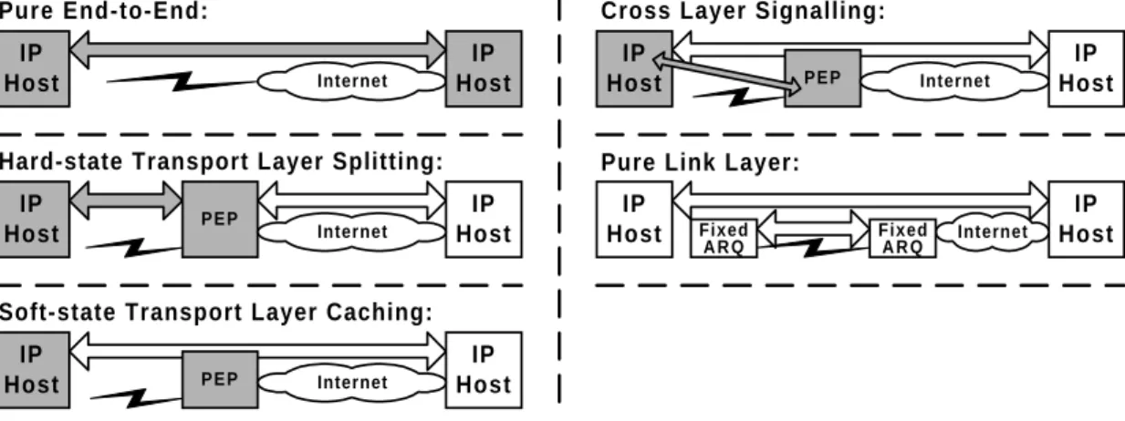
Related work suggests solutions that are either pure end-to-end (e.g., [SF98]), leaving unex-ploited the potential of link layer error control schemes to optimize end-to-end performance, or only suggest link layer mechanisms (e.g., [BBKT97], [ES98], [Kar93]), none of which is capa-ble of solving all inefficient interactions with end-to-end control schemes. Most prior work (e.g., [BB95], [BK98], [BS97], [DMT96], [HK99], [KRLKA97]), however, suggests

Perfor-mance Enhancing Proxies (PEPs) that couple link layer and end-to-end control schemes to

solve inefficient cross-layer interactions. These solutions violate the fundamental design prin-ciple in data communications, protocol layering, by requiring access to transport layer headers by the PEPs. Our approach is fundamentally different in that we do not require - in fact, we argue against - such cross-layer couplings. The key advantages of our solution over PEP-based approaches are (A) its independence from transport (or higher) layer protocol semantics mak-ing it a “non-TCP-specific” solution, (B) the possibility of co-existence with network layer encryption, e.g., IPsec [RFC2401], and (C) that no per-flow state needs to be maintained in the network making it more scalable. The main contributions of this dissertation are the following:

1. The new concept of flow-adaptive wireless links and its application for fully-reliable flows. This work has been published in [LR99], [LRKOJ99], and [LKJK00].

2. Two new mechanisms for reliable end-to-end protocols, the Eifel algorithm and the Eifel

retransmission timer. The former has been published in [LK00] while the latter is

described in [LS99]. We have implemented both mechanisms for TCP, and refer to that implementation as TCP-Eifel that we have made publicly available [Lud99c].

(9)

The remainder of this chapter describes and motivates the outline of this dissertation.

Chapter 2 provides required background. After we introduce related terminology in Section 2.1, the following three sections review those functions of the control schemes shown in Figure 1-1 that are relevant for our studies. Since all our “real-world” measurements in wire-less networks were carried out using GSM-CSD, the Circuit-Switched Data (CSD) service implemented in the Global System for Mobile communications (GSM), we explain that net-work in more detail. In Section 2.5 we describe all inefficient cross-layer interactions in wire-less networking that are known in literature. Related work is reviewed and evaluated in Section 2.6. We present a brief motivation and outline of the approach taken in this dissertation in Section 2.7.

Chapter 3 explains the analysis methodology we applied and the tools we developed to obtain the results presented in Chapter 4 and Chapter 5. We first motivate why we have mostly chosen a measurement-based analysis approach. In Section 3.1, we then explain the methodology we use in Section 4.3 to evaluate the benefit of link layer error recovery for reliable flows. We explain how we capture and analyze the error characteristics of the GSM-CSD wireless link. Our ReTracer tool is described, which we developed to reverse-engineer target metrics such as throughput given certain parameters like the link layer frame size. In Section 3.2, we explain the methodology we use in Section 4.2 to detect inefficient cross-layer interactions between TCP and the link layer error control implemented in GSM-CSD. We describe the tools we developed for that purpose: rlpdump, an event logging tool for the reliable link layer col implemented in GSM-CSD, and MultiTracer, used to correlated events on different proto-col layers. There we also explain how to interpret TCP trace plots, which we often use to illus-trate certain effects, problems, or solutions. In Section 3.3, we explain the methodology we use in Section 5.1 to study the problem of competing error recovery for the case of TCP, and to develop the Eifel algorithm in Section 5.2 that eliminates this problem. We explain how we used the hiccup tool that we developed to reproduce inefficient cross-layer interactions in a “non-wireless” but controllable network environment. In Section 3.4, we explain the method-ology we use in Section 5.3 to study and reveal the problems of TCP-Lite’s retransmission timer. We use the same model in Section 5.4 to develop the Eifel retransmission timer that eliminates those problems. We explain the model that we developed to analyze those end-to-end retransmission timers, and the measurement setup we used to validate the correctness of the model. In Section 3.5, we provide a summary of the chapter.

Chapter 4 introduces the concept of flow-adaptive wireless links, and validates it for fully-reli-able flows. In Section 4.1, we explain that concept and discuss its deployment concerns, and possible implementation alternatives. The key idea is that network end-points use the IP layer as a level of indirection through which their QoS requirements are signalled to each link layer along the path, on a per packet basis. This allows for a (wireless) link layer to adapt its error

(10)

control schemes to meet those requirements while minimizing radio resource consumption. We argue against and illustrate the problems of running low link layer error recovery persistency for fully-reliable flows. In Section 4.2, we verify through measurements, that our solution of flow-adaptive wireless links eliminates all known inefficient cross-layer interactions except for the problem of competing error recovery. This study also delivered early indications that the retransmission timer implemented in TCP-Lite is too conservative. In Section 4.3, we show how the GSM-CSD wireless link can be adapted to optimize the end-to-end performance of bulk data flows. We use this case study to demonstrate that link layer error recovery over wire-less links is essential for reliable flows to optimize their end-to-end performance. In Section 4.4, we provide a summary of the chapter.

Chapter 5 provides solutions to the remaining problems we identified in Chapter 4. In Section 5.1, we identify the retransmission ambiguity in TCP as the root of the problems caused by competing error recovery. In Section 5.2, we develop the Eifel algorithm that uses extra information in the TCP acknowledgements to resolve the retransmission ambiguity, and show how this is used to eliminate those problems. The Eifel algorithm only requires changes to the TCP sender implementation, not to the protocol itself. Thus, given this backwards com-patibility and the fact that it does not change TCP’s congestion control semantics, the new algorithm can be incrementally deployed. In Section 5.3, we analyze TCP-Lite’s retransmis-sion timer, and reveal a number of problems related to its definition and implementation. This explains why we had suspected that this timer is too conservative. In Section 5.4, we then pro-pose an alternative retransmission timer, which we call the Eifel retransmission timer, that eliminates those problems. We demonstrate that the Eifel retransmission timer is a more pre-cise predictor of an upper bound for the path’s RTT. Combining both, the Eifel algorithm and the Eifel retransmission timer, we propose a new approach to designing retransmission timers. The idea is to let the timer become increasingly aggressive while adapting it to the measured fraction of spurious timeouts. We validated the correctness of our analysis by showing that the model- and the measurement-based approach leads to the same results. In Section 5.5, we pro-vide a summary of the chapter.

Chapter 6 concludes this dissertation by summarizing our main results and outlining related but unsolved research problems that merit further exploration.

(11)

CHAPTER 2

Background

In this chapter, we explain the relevant technologies and related work for the background required in subsequent chapters. The first three sections describe the “three corners” of the tri-angle shown in Figure 1-1. In Section 2.5, we define the central problem (the center of Figure 1-1) this dissertation addresses. In Section 2.6, we briefly explain how related work has approached the problem, and provide an evaluation of the proposed solutions. In Section 2.6, we briefly motivate and outline the approach developed in the remainder of this dissertation.

2.1 Terminology

The Internet is an inter-connection of networks. A network connects hosts and networks are interconnected via routers. Communication in the Internet is based on the Internet Protocol

(IP), a network layer protocol defined by [RFC791], referred to as IP-Version 4 (IPv4), and

alternatively by [RFC2460], referred to as IP-Version 6 (IPv6). A protocol data unit in IP is called a packet, consisting of an IP header followed by transport layer data1. The transport layer data may (in theory) be up to 64 KBytes large. The default size of the IP header is 20 bytes, and with option fields may be up to 60 bytes. The IP protocol is connection-less and as such does not guarantee in-order delivery of packets. That is, the sequence of packets as generated by the source does not need to be preserved when the packets are delivered to the destination. That responsibility is left to higher layer protocols such as the Transmission

Con-trol Protocol (TCP). In particular, packets belonging to the same connection may take different

routes to the destination and in practice sometimes do [Pax97d].

(12)

In most cases, a host is a general purpose computer but it may also be a specialized appliance. Examples of a network are an Ethernet (multi-access), a dial-up line provided by a fixed or wireless telephone system (point-to-point), or a direct cable that connects two hosts via their serial line interfaces (point-to-point). The network that connects two hosts, two routers, or a host and a router is also called a link or hop. Communication across a link is provided by a link layer protocol. A protocol data unit in a link layer protocol is called a frame. A host connects to a link via a network interface (or just interface). Each interface on a host has an interface address that is unique in the corresponding network and an IP address that is unique in the Internet. The source and destination IP addresses are part of the IP header. The receiving IP layer uses the protocol identifier that is also part of the IP header to decide to which transport protocol, e.g., TCP, it is supposed to deliver the packet’s payload. Transport layer service is provided through a port identified by a port number which is unique only in combination with an IP address and a protocol identifier. The source and destination port numbers are part of a transport protocol header.

A series of links connecting two hosts is called a path. Communication between two processes at each end of a path is referred to as end-to-end communication. Such a process is generally called a network end-point (or just end-point). End-to-end communication is provided by net-work (IP), transport and (optionally) application layer protocols, so-called end-to-end proto-cols. Thus, a network end-point can be a sending/receiving network (IP), transport or applica-tion layer, or a sending/receiving applicaapplica-tion.

An end-to-end stream of packets identified by the source and destination IP address, the source and destination port number, and the protocol identifier, is referred to as a flow. For example, the packets sent by a TCP sender to a TCP receiver corresponds to a flow; a TCP-based flow. A network end-point is tied to one specific flow and each flow has two network end-points, a sending and a receiving network end-point. Hence, a property of a flow may also be associated with a network end-point and vice versa. When speaking of such properties, we use the terms

network end-point and flow interchangeable.

A flow’s bottleneck link is the link on which the bandwidth available to the flow is the lowest of all links in the path. That bandwidth is also referred to as the flow’s available bandwidth as it limits the end-to-end throughput that the flow may provide. The flow’s available bandwidth can be very dynamic depending how many flows share the bottleneck link and how much of the bottleneck link’s bandwidth those flows consume. We define as the packet transmission

delay the time it takes to successfully transmit a packet over a given link excluding any

queue-ing delay that may occur before the initial transmission of the packet. A flow’s round trip time

(RTT) (sometimes also called the path’s RTT) is the time it takes to send a packet from one

net-work end-point to the other, get it processed at the receiving end-point, and send another packet back to the end-point that sent the initial packet. A flow’s RTT varies dynamically,

(13)

depending on such factors as packet size (transmission delays), queueing delays the packets experience in the network, and processing required at the receiving end-point1. The packets a network end-point sends within the flow’s RTT is called a flight of packets (or just flight). Those packets are also referred to as the packets a network end-point or flow has in flight. The number of packets a network end-point has in flight is called the flow’s load2.

Link layer and end-to-end protocols3 have the following functions in common, not all of which have to be implemented (see [Tan89] or [Ste94] for more detail). We use the term user process to refer to the process that uses the protocol being described.

• Framing ensures that data units passed by a sending user process to a protocol are deliv-ered as the same data units to the receiving user process. For example, if implemented at the link layer, it allows the receiving link layer to recognize the beginning and the end of an IP packet. This enables the receiving link layer to deliver each IP packet as a single unit to the receiving IP layer, i.e., the receiving user process.

• Flow control to prevent a fast sender to overflow a slow receiver.

• Error detection ensures that a protocol data unit received in error is discarded and is not delivered to the receiving user process. This function is provided by adding a checksum to each protocol data unit that the receiving protocol layer verifies.

• Error recovery - also known as Automatic Repeat reQuest (ARQ) - requires error detection and ensures that lost protocol data units and protocol data units received in error are retransmitted. We define as error recovery persistency the maximum number of retransmissions an error recovery scheme performs for a single protocol data unit before it is discarded. Alternatively, error recovery persistency may be defined as the maximum permissible delay that the error recovery scheme may introduce for a single protocol data unit before is discarded.

• In-order delivery ensures that the sequence of the data units passed by a sending user pro-cess to a protocol is preserved when those data units are delivered to the receiving user process.

• Removal of data that might have been duplicated during transmission by the protocol. A protocol provides reliable service if it implements the latter five functions. It provides

unre-liable service if it implements error detection but not necessarily error recovery. It provides transparent service if it does not implement error detection. Either service may or may not sup-1. For example, also including the delayed-ACK timer of 500 ms that may be used in TCP [RFC1122].

2. Some of those packets might have left the network already but because of the feedback delay (the RTT), the sending net-work end-point might not yet be aware of it. Also note, that the feedback might be provided explicitly, e.g., through ACKs as in TCP (see Section 2.2.1), or implicitly through (RTT and packet loss rate) measurement reports provided by the receiv-ing network end-point as done for “TCP-friendly” flows (see Section 2.3.3).

(14)

port framing. A service that does not support framing is referred to as a byte stream service. Further, reliable protocols need to establish a connection at the beginning of each instance of communication. A connection is required to establish and maintain common protocol state (e.g., initial sequence numbers, flow control windows) between the sending and the receiving protocol layer.

The fact that IP does not need to preserve the packet order also allows for link layer protocols that provide reliable service to perform out-of-order delivery of correctly received IP packets, i.e., to not implement the above mentioned in-order delivery function. This provides for more memory-efficient link layer implementations. We still regard such a link layer protocol as pro-viding reliable service, but make it explicit in the text when referring to that case.

We further distinguish between fully-reliable and semi-reliable service. When the error recov-ery persistency is reached, a protocol providing fully-reliable service terminates the connection (discards the common connection state) and indicates that event to the sending and the receiv-ing user process. Those processes then “know” that data was lost and may or may not decide to re-initiate their communication. A protocol that provides semi-reliable service, on the other hand, does not terminate the connection when its error recovery persistency is reached, and does not indicate that event to the sending and the receiving user process. Instead, it just dis-cards the corresponding protocol data unit and resumes transmission with the next one in sequence. We also use the terms (fully- or semi-) reliable, unreliable, or transparent in associa-tion with the term protocol depending on which service it provides, and with the term flow depending on which service the flow provides to the application. For example, the flow gener-ated by a reliable multicast protocol, like [FJLMZ97], is considered reliable even if UDP is the underlying unreliable transport protocol. A flow generated by TCP is an example of a fully-reliable flow.

A link layer protocol that provides service directly to IP needs to implement framing and is called a framing protocol. Throughout this text we only refer to one framing protocol which is the Point-to-Point Protocol (PPP) [RFC1661] commonly used on dial-up and direct cable links. By default, PPP provides an unreliable service1. A framing protocol defines the link’s

Maximum Transmission Unit (MTU), i.e., the size in bytes of the largest IP packet that can be

transmitted on that link. The smallest MTU of all links of a path is called the path MTU. The IP layer includes a fragmentation function, referred to as IP fragmentation [RFC1122], that is used in case a packet is larger than the outbound link’s MTU. IP fragmentation may be per-formed by the sending host’s IP layer or any router’s IP layer. If an IP packet needs to be frag-mented, it is divided into smaller fragments and a copy of the IP header is prepended to each fragment. A fragment number is inserted into each of those headers so that the destination IP

(15)

layer can perform the reassembly of the original IP packet. IP fragments are transmitted and routed as regular IP packets.

We further classify flows according to the type of traffic they carry. Bulk data flows are gener-ated by applications that need to transfer “large” amounts of data (e.g., file transfer or e-mail). The main Quality of Service (QoS) requirement of such flows, more precisely the QoS require-ment of the corresponding application, is to maximize throughput, i.e., to transfer the entire data as fast as possible, while the end-to-end delay of an individual packet is less important1. We also speak of a bulk data transfer in this respect. Interactive flows are used for transac-tional (request/response-style) communication (e.g., remote terminal or banking applications). The main QoS requirement of such flows is to minimize the end-to-end delay of the packets belonging to a transaction, i.e., a low user level response time, while the end-to-end throughput that the flow may provide is less important. Bulk data and interactive flows are usually based on an end-to-end protocol that provides a fully-reliable service (e.g., TCP). Real-time flows, on the other hand, are usually based on an unreliable end-to-end protocol, e.g., the User

Data-gram Protocol (UDP) [RFC768]. They are generated by applications that are delay-sensitive

(e.g., audio and video applications). An important class of real-time flows in the Internet are

rate-adaptive real-time flows, e.g., those based on the Real-Time Transport Protocol (RTP)

[RFC1889]. Applications that operate on such flows can adapt (to certain degrees) the output rate of their source codecs to the flow’s available bandwidth. A comprehensive discussion of flow types and their QoS requirements can be found in [She95].

A packet loss is the event that a packet is sent into the Internet but does not reach the destina-tion. A packet can get lost because it is dropped due to congestion (see Section 2.3) at an inter-face’s in- or outbound buffer, or it is discarded due to transmission error by a link layer error detection function (see Section 2.4). We call the former event a congestion loss and the latter event an error loss.

2.2 End-to-End Error Recovery with TCP

2.2.1 Basic Operation

The basic functionality of TCP is defined by [RFC793], [RFC1122], and [RFC2581]. TCP extensions have been defined by [RFC1323], [RFC2018], and [RFC2481]2. Those six

recom-1. In theory, it would not matter in a file transfer if the first packet reached the destination last. What usually matters is that the file transfer is completed in the shortest amount of time. In practice, the transport layer receive socket buffer required for packet re-sequencing places a limit on the maximum per packet delay that is tolerable without affecting performance. This limit is nevertheless low.

(16)

mendations have been proposed over a time frame of almost twenty years. During this time numerous TCP implementations for various operating systems have been developed. Some of these predate the more recent recommendations, and not every desirable TCP feature has been specified. Moreover, some TCP implementations are incorrect due to logic errors, misinterpre-tations of the specification, or conscious violations to gain better performance [Pax97b]. Con-sequently, many different “TCPs” exist today. Throughout this dissertation we refer to the so-called TCP-Lite implementation for the Berkeley Software Distribution (BSD) operating sys-tem documented in [WS95]. In the Internet research community, it is the current de facto stan-dard for TCP implementations. It has been ported to various operating systems running daily on hundreds of thousands of servers and clients on the Internet. We omit the qualifier “-Lite” when discussing TCP in general as specified by the above listed recommendations.

TCP is a transport layer protocol that provides a fully-reliable byte stream service. It exchanges data with the user process through shared memory, so-called (send and receive)

socket buffers. The size of TCP’s socket buffers are usually determined by default settings of

the operating system; commonly 8 or 16 KBytes. A protocol data unit in TCP is called a

seg-ment, consisting of a TCP header followed by application layer data. The default size of the

TCP header is 20 bytes, and with option fields may be up to 60 bytes. Each segment is trans-mitted as a separate packet, and the receiving IP layer delivers it as a single unit to the receiv-ing TCP layer. Thus, a segment does not require (begin/end) delimiters. Each byte in the appli-cation layer byte stream corresponds to a unique sequence number in a TCP connection. The header of each segment carries the sequence number of the first byte in the segment. The size of the application layer payload is variable but may not be larger than the Maximum Segment

Size (MSS)1. The default MSS is 536 bytes derived from the default MTU size (576 bytes) which leaves space for default size TCP and IP headers. The MSS to be used by the TCP sender is usually announced by the TCP receiver during connection establishment through the

MSS option in the TCP header. Nevertheless, it is limited by the outbound link’s MTU (minus

the size of the TCP/IP header). Alternatively, the sender may use the path MTU discovery pro-cedure [RFC1191] to derive an appropriate MSS. The specification [RFC793] arbitrarily assumes a value of 2 minutes for the Maximum Segment Lifetime (MSL). The MSL controls the maximum rate at which segments may be sent before the sequence numbers wrap around.

A TCP receiver sends positive acknowledgements (ACKs) for segments that are received cor-rectly and in-order and duplicate acknowledgements (DUPACKs) for segments that are received correctly but out-of-order. No feedback is provided for segments received in error. ACKs may be generated for every segment, or for every other segment if the delayed-ACK mechanism [RFC1122] is used. DUPACKs may not be delayed. Both types of acknowledge-ments contain the so-called ACK number that is next sequence number that the TCP receiver

1. Note the slight illogicality: Although both the TCP header and the application layer payload together constitute a segment, the segment size, in particular the MSS, only applies to the payload.

(17)

expects to receive. A DUPACK contains the same ACK number as the last sent ACK. Thus, a DUPACK does not convey which segment was received correctly (unless Selective Acknowl-edgement Options [RFC2018] are used). The segments or bytes the TCP sender has sent and which are waiting to be acknowledged are called outstanding.

Two different error recovery strategies have been specified for TCP: (1) timeout-based retrans-mission, and (2) DUPACK-based retransmission. In the latter case a retransmission - a so-called fast retransmit - is triggered when three1 successive DUPACKs with the same ACK number have been received independent of the retransmission timer [Jac90a]. Section 2.2.2 provides a detailed description of TCP’s retransmission timer. TCP’s error recovery is fairly persistent. It retransmits a single segment twelve times which corresponds to roughly 9 minutes before the connection is aborted.

Flow control is provided through the well-known sliding window mechanism. ACKs sent by the TCP receiver carry the advertised window, which limits the number of bytes the TCP sender may have outstanding at any time. The advertised window (usually) corresponds to the size of TCP receiver’s receive socket buffer. End-to-end protocols that implement sliding win-dow flow control, like TCP, share an important self-clocking property [Jac88]. We explain this with Figure 2-1 (a modified version of a figure taken from [Jac88]) showing a schematic repre-sentation of a sender and a receiver on high bandwidth networks connected by a slow link, the bottleneck link, that is error-free. The vertical dimension is bandwidth, the horizontal dimen-sion is time. Each of the shaded boxes is a packet. Because “bandwidth x time = bits”, the area of each box is the packet size. Thus, a packet on the slow link (occupying less in the vertical

1. Note, that most implementations define a DUPACK-Threshold. However, that threshold is commonly set to three.

T_B T_B T_B T_B T_B

Sender

Receiver

queued packets pipe capacity

(18)

dimension) has to spread more in time (occupying more in the horizontal dimension). Figure 2-1 shows the ideal case in which a single sender fully utilizes the non-shared bottle-neck link with a fixed bandwidth and always sends fixed size segments. In that case the ACK inter-arrival time at the sender is constant and equal to the packet transmission delay over the bottleneck link, T_B. This constant stream of returning ACKs is referred to as the ACK clock. The arrival of an ACK “moves the sliding window to the right” by one segment and “clocks out” a new segment. Consequently, for every packet that leaves the bottleneck link, a new packet arrives.

2.2.2 TCP-Lite’s Retransmission Timer

While data is outstanding the TCP sender samples the path’s RTT by timing the difference between sending a particular segment and receiving the corresponding ACK. Older TCP implementations only time one segment per RTT, whereas newer implementations use the timestamp option [RFC1323] to time every segment. Timing every segment allows much closer tracking of changes in the RTT. When using the timestamp option, the TCP sender writes the current value of a “timestamp clock” into a 12 bytes option field in the header of each outgoing segment. The receiver then echos those timestamps in the corresponding ACKs according to the rules defined in [RFC1323]. When receiving an ACK the TCP sender deter-mines the RTT by calculating the difference between the current value of its “timestamp clock” and the timestamp echoed in the ACK. In the context of TCP, we speak of “the RTT” when referring to the RTT of the last segment for which the sender received the ACK, independent of whether the sender had timed that segment to derive the RTT.

We refer to the RTT sampling rate as the number of RTT samples the TCP sender captures per RTT divided by the TCP sender’s load. In case the TCP sender times every segment and the TCP receiver acknowledges every segment, the RTT sampling rate is 1. If the TCP sender times every segment and the TCP receiver acknowledges every other segment (delayed-ACK), the RTT sampling rate is 1/2. If the TCP sender only times one segment per RTT, the RTT sam-pling rate is the reciprocal of the TCP sender’s load. The closer the RTT samsam-pling rate is to 1 the more accurately the TCP sender measures the RTT.

The retransmission timeout value (RTO) is the time that elapses after a packet has been sent until the sender considers it lost and therefore retransmits it. This event is called a timeout. The RTO is a prediction of the upper limit of the RTT which - especially on an end-to-end path through the Internet - may vary considerably for various reasons. The time that remains until the timeout for a packet occurs is maintained by the retransmission timer state (REXMT). Thus, the RTO is the REXMT’s initial value. We use the term retransmission timer to refer to the combination of REXMT and RTO.

(19)

The retransmission timer is a key feature of a reliable transport protocol like TCP. It can greatly influence end-to-end performance. A too optimistic retransmission timer often expires prematurely. Such an event is called a spurious timeout. It causes unnecessary traffic, so-called

spurious retransmissions, reducing a connection’s effective throughput. In TCP, timeouts also

trigger congestion control (explained in Section 2.3.2), that may additionally reduce the end-to-end throughput. A retransmission timer that is too conservative may cause long idle times before the lost packet is retransmitted. This can also degrade performance. This is obvious for interactive flows. But it also affects bulk data transfers whenever the TCP sender has exhausted the window limiting the number of outstanding segments before the retransmission timer expires.

In the following, we refer to TCP-Lite’s retransmission timer as the Lite-Xmit-Timer. We use the index L (Lite) as a qualifier for a metric when referring to its definition or implementation. We omit that qualifier when discussing a particular metric in general. The following set of equations define RTO_L [JK92]. In its implementation, RTO_L is updated every time the TCP

sender completes a new RTT measurement, denoted as RTT_Sample.

SRTT is the so-called smoothed RTT estimator. SRTT_L is a low-pass filter that keeps a memory of a connection’s RTT history with a fixed weighing factor of 7/8. DELTA_L is the difference between the latest RTT_Sample and the current SRTT_L. RTTVAR is the so-called smoothed RTT

deviation estimator. Through RTTVAR, the RTO accounts for variations in RTT. RTTVAR_L is a low-pass filter that keeps a memory of a connection’s RTT deviation history with a fixed weighing factor of 3/4. We refer to the constants 1/4 and 1/8 as the estimator gains and to the constant 4 as the variation weight. Little motivation other than implementation efficiency is provided in [JK92] for this particular set of constants.

REXMT and RTO are maintained in multiples of ticks, i.e., some fraction of a second that is operating system dependent. This is also referred to as the timer granularity. REXMT_L is based on a so-called heartbeat timer provided by the BSD operating system implementing a timer granularity of 500 ms. The heartbeat timer expires every 500 ms, triggering a specific interrupt routine that updates the REXMT_L (decrements it by one tick) of each active TCP connection. This is done independent of whether one of those REXMT_L would actually go to zero or not. If

DELTA_L = RTT_Sample–SRTT_L SRTT_L SRTT_L 1 8 ---×DELTA_L + = RTTVAR_L RTTVAR_L 1 4 ---×(DELTA_L –RTTVAR_L) + =

(20)

REXMT_Lwas initialized with a value of one it could expire anywhere between 0 - 1 tick, because the initialization event is out of phase with the heartbeat timer. Therefore, a minimum of 2 ticks is required for RTO_L to prevent spurious timeouts in case

evaluates to one.

We call the time that has elapsed since a segment was sent the age of a segment. Likewise we refer to the oldest outstanding segment as that segment in the TCP sender’s send socket buffer with the highest age. That segment also carries the lowest sequence number of all outstanding segments. It is the segment that gets retransmitted when REXMT expires. TCP-Lite maintains a single REXMT per TCP connection. The following equation defines REXMT_L. When a seg-ment is sent and REXMT_L is not active, it is started (initialized with RTO_L). When an ACK arrives that acknowledges the oldest outstanding segment and more segments are still out-standing, REXMT_L is re-initialized with RTO_L.

We briefly summarize related work concerning the Lite-Xmit-Timer. Karn’s algorithm [KP87] must be implemented in TCP [RFC1122]. It prevents a clamped retransmission timer by ignor-ing the RTT_Samplederived from a retransmitted segment and doubling the RTO (exponential

timer backoff) up to a maximum of two times MSL, i.e., 240 seconds, each time REXMT

expires for the same segment. This makes it possible to eventually collect a valid RTT_Sample again. Otherwise the sender might get stuck retransmitting the oldest outstanding segment while REXMT is clamped at too low a value. The authors of [BP95b] remove an inaccuracy in the implementation of RTO_L that made it more conservative then intended in its definition. This has been updated accordingly in later TCP implementations (e.g., in the FreeBSD operat-ing system). Through trace-driven simulation, the Lite-Xmit-Timer and some of its variations are evaluated in [AP99] against a large set of real measurements. The authors conclude that the RTO minimum (2 x ticks, i.e., 1 second) dominates the performance of the Lite-Xmit-Timer and that its performance can be further increased when a timer granularity of 100 ms or less is implemented. However, the study also concludes that the estimator gains and the RTT sam-pling rate have little influence on the Lite-Xmit-Timer’s performance. We disagree with the latter conclusion and show in Section 5.3.2 that in fact the opposite is the case.

2.2.3 TCP/IP Header Compression

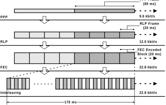
Although, TCP/IP header compression [RFC1144], [RFC2507] is a link layer mechanism, it has a lot to do with TCP’s end-to-end error recovery. It is commonly implemented as part of a link’s framing protocol, and is used to reduce the per packet overhead transmitted over the link. In the common case, a default size TCP/IP header of 40 bytes is compressed to 4 bytes. This

SRTT_L+4×RTTVAR_L

(21)

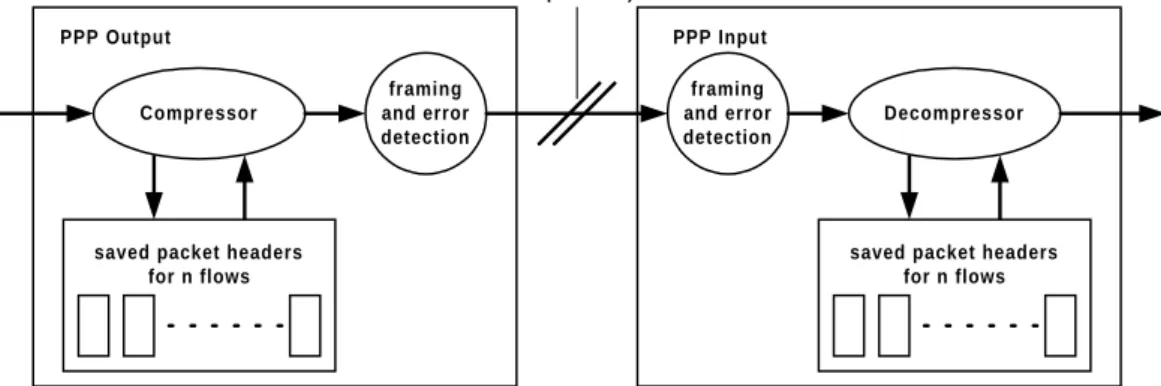
compression ratio is possible because - apart from the sequence number, the ACK number, and the checksums (one for the IP header and one for the TCP segment) - not much changes in the headers from packet to packet of the same flow. The advantages of header compression are cost savings on links with volume based charging and increased link throughput. For example, if the link’s MTU is 296 bytes - a size commonly used on dial-up links - TCP/IP header com-pression increases the link’s achievable throughput by more than ten percent. Figure 2-2 (taken from [RFC1144]) sketches the location of the compressor and the decompressor in the packet stream.

TCP/IP header compression is a differential encoding (also called delta encoding). After the first TCP/IP header of a flow has been transmitted uncompressed, only the encoded difference to the preceding header, the delta, is transmitted as the header of a packet. The decompressor derives the uncompressed header by applying the delta to the stored header of the packet that was last received for that flow. As with other differential encoding schemes, TCP/IP header compression relies on the fact that the deltas (more precisely the packets carrying the deltas) are not lost or reordered on the link between compressor and decompressor. A lost delta (packet) will lead to a series of false headers being generated by the decompressor, yielding

TCP/IP packet

saved packet headers for n flows Compressor framing and error detection PPP Output framing and error detection PPP Input Decompressor

saved packet headers for n flows

TCP/IP packet Simplex serial link

(1/2 of real, full duplex link)

Figure 2-2: Location of the TCP/IP header de-/compressor in the packet stream.

100100 100150 100200 100250 De- Compress Compress D-50 D-50 D-50 D-50 Transfer D-50 D-50 D-50 D-50 100100 100150 100200 100050 D-50 D-50 100050 100000 100000 100000 100000

(22)

TCP segments that have to be discarded at the TCP receiver because of checksum errors. This is sketched in Figure 2-3 showing an initial sequence number of 100,000 which increases by 50, the delta, from packet to packet. To resynchronize the compressor and the decompressor, [RFC1144] and [RFC2507] require that the TCP/IP headers of packets containing a retransmit-ted segment may not be compressed. Thus, once a delta is lost, an entire flight of segments is lost and has to be retransmitted. Even worse, since the TCP receiver does not provide feedback for erroneous TCP segments, the TCP sender is forced into a timeout. We have measured this effect and further discuss this issue in Section 4.2.3. [RFC1144] and [RFC2507] differ in their robustness against lost deltas. Whereas [RFC1144] cannot tolerate a single lost delta (the case shown Figure 2-3), [RFC2507] can tolerate the loss of a single lost delta - using the twice

algo-rithm - but also loses synchronization once two deltas are lost back-to-back.

It is worth pointing out that header compression is an example of layer violation: a particular layer (in this case the link layer) inspects and interprets a higher layer’s headers. Typical cases of layer violation are nodes in the network that require access to the headers of an end-to-end protocol.

2.3 End-to-End Congestion Control in the Internet

2.3.1 Objectives and Principles

A best-effort network like the Internet does not have the notion of admission control or resource reservation to control the imposed network load, i.e., the total number of packets that reside within the network. A best-effort network under high network load is called congested. If the network is in this state, host and/or router network interface buffers may overflow caus-ing packets to be lost (dropped), i.e., congestion losses. Network end-points sharcaus-ing a best-effort network need to respond to congestion by implementing congestion control to ensure network stability. Otherwise, the network may be driven into congestion collapse: the network load stays extremely high but throughput is reduced to close to zero [RFC896]. Thus, the objective of end-to-end congestion control is for network end-points to estimate (by probing the network) their available bandwidth while ensuring network stability.

In the following, we give a general description of congestion control in the Internet, and intro-duce related terminology. A more detailed description of these terms and concepts is provided in Section 2.3.2, where we explain how congestion control is implemented in TCP.

A congestion control scheme has three basic elements: (1) the network must have a congestion

(23)

network end-points must have a policy to decrease their load on the network in response to the congestion signal, and (3) the network end-points must have a load increase policy in times when the congestion signal is not received as this may indicate that more bandwidth has become available at the bottleneck link. The latter is also referred to as probing (for

band-width). The key issue is the congestion signal. One distinguishes between explicit congestion

signals issued by the network and implicit congestion signals inferred from certain network behavior by the network end-points. Routers in today’s Internet do not issue explicit conges-tion signals1, although this might be implemented in the future [RFC2481] (see Section 2.3.3). Two approaches have been discussed for network end-points relying on an implicit congestion signal: delay-based [Jai89], [BP95a] and loss-based [Jac88], [Jac90a]. However, it is often not possible to draw sound conclusions from network delay measurements (e.g., see [BV99]). In particular, it is difficult to find characteristic measures such as the path’s minimum RTT as required by [BP95a]. This may be due to route changes [Pax97d] or persistent congestion at the bottleneck link. Consequently, “packet loss” is the only signal that network end-points can confidently use as an indication of congestion. It is implemented either as a direct trigger (see Section 2.3.2) based on the detection of a lost packet, or an indirect trigger, based on a per-ceived packet loss rate (see Section 2.3.3) to reduce a flow’s load. Such network end-points and their corresponding flows are loss responsive. In this dissertation, we only deal with loss responsive flows. We often omit the qualification “loss responsive” when talking of flows. In the absence of an explicit congestion signal, an additive increase and a multiplicative decrease policy is required in an heterogeneous environment like the Internet to converge to network stability [Jac88], [CJ89].

We define as the flow’s pipe capacity the minimum number of packets a flow needs to have in flight, i.e., the minimum load, to fully utilize its available bandwidth. Packets of a flow’s load exceeding the flow’s pipe capacity are queued in the network (see Figure 2-1). They contribute to network congestion and an increased end-to-end delay, which also affects the flow’s own RTT. Ideally, a network end-point would not increase its load beyond its flow’s pipe capacity. However, this is impossible with a congestion control scheme that only relies on an implicit congestion signal. With such a scheme the network end-points treat the network as a “black box”, but the flow’s pipe capacity can only be known by “looking into the black box”.

A network end-point or flow is network-limited if its load is limited by congestion control. This property is commonly associated with bulk data and rate-adaptive real-time flows, rarely with interactive flows. Whether a network-limited flow fully utilizes its available bandwidth depends on the number of packets the flow may have in flight beyond its pipe capacity, i.e., the number of packets that may be queued in the network before a packet is dropped due to

(24)

gestion. A network end-point or flow that is not network-limited is called application-limited. The load of such flows is limited by the rate at which the sending application can generate data and/or the rate at which the receiving application can consume the data. Examples include interactive TCP-based flows and rate-adaptive real-time flows of which the corresponding application can run its maximum rate (highest quality) source codec. Whether an application-limited flow fully utilizes its available bandwidth depends on the rate at which the sending/ receiving application generates/consumes data.

2.3.2 Congestion Control in TCP

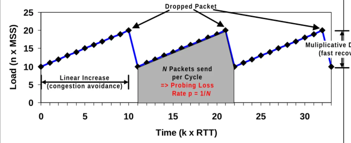
The two error recovery strategies used in TCP (see Section 2.2.1) are coupled with TCP’s con-gestion control scheme [Jac88], [Jac90a], [RFC2581] in the following way. After a timeout-based retransmission, the TCP sender decreases its load to one segment (see the 27th RTT in Figure 2-4). It then enters the slow start phase during which it increases the load exponentially until the load reaches one half of its value before the timeout (see the 30th RTT in Figure 2-4). The TCP sender then enters the congestion avoidance phase, where it increases the load lin-early. The congestion avoidance phase is sometimes also called the probing phase because the TCP sender is probing the network for more bandwidth. After a DUPACK-based retransmis-sion, the TCP sender halves its load (see the 6th, 11th, and 18th RTT in Figure 2-4), and imme-diately enters the congestion avoidance phase. This behavior is justified because a packet loss usually indicates congestion somewhere along the path and a timeout indicates more severe congestion. Load above the “Pipe Capacity” line in Figure 2-4 is queued in the network. The implementation of this congestion control scheme is intertwined with TCP’s window-based flow control scheme through the use of two sender-side state variables: the slow start

threshold (ssthresh) and the congestion window (cwnd), which are both measured in bytes

[Jac88]. A TCP sender is never allowed to have more bytes outstanding than the minimum of the advertised window and the congestion window. That is, a TCP sender’s load is limited by

0 2 4 6 8 10 12 14 16 18 1 3 5 7 9 11 13 15 17 19 21 23 25 27 29 31 33 Tim e (k x RTT) Load (n x MSS) Pipe Capacity 3rd DUPACK 3rd DUPACK 3rd DUPACK Timeout Slow Start Threshold Reached

(25)

the flow control imposed by the receiver and by the congestion control (implicitly) imposed by the network. In the latter case a TCP flow is called network-limited as defined above, in the former case it is called receiver-limited. In addition, a TCP sender’s load is limited by the size of the TCP sender’s send socket buffer that is used to hold outstanding segments in case they need to be retransmitted. Such TCP flows are called sender-limited. Because the socket buffer sizes are controlled by the application, we consider receiver- and sender-limited TCP-based flows as special cases of application-limited flows.

Figure 2-5 shows the finite state machine1 implemented for the TCP sender that results in the congestion control behavior depicted in Figure 2-4. When a connection is established, ssthresh and cwnd are initialized to 64 KBytes and MSS, respectively, and the connection enters the slow start phase. In that phase every ACK increases cwnd by one MSS causing an exponential increase in cwnd over RTT, i.e., cwnd is doubled per RTT2.

As soon as cwnd exceeds ssthresh, the connection enters the congestion avoidance phase. In that phase every ACK increases cwnd by MSS2/cwnd. This causes a linear increase in cwnd over RTT, i.e., cwnd is increased by one MSS per RTT3. When the third DUPACK is received that triggers the fast retransmit (either during slow start or during congestion avoidance), one half of the current value of cwnd is stored in ssthresh4, and the connection enters the fast

recovery phase [Jac90a].

The purpose of the fast recovery phase is to reduce the load on the network by one half. This is accomplished by suppressing the transmission of new segments for the first half of the

return-1. To not confuse the diagram, we do not show the end state. For a complete finite state machine a transition (“disconnect”) from each of the states shown in the diagram to the end state must be added.

2. Such an ACK clocks out two segments: one because the sliding window “moved right” by one segment and another one because cwnd increased by one segment. In case delayed-ACKs are used, even three segments are clocked out because in that case, the sliding window “moved right” by two segments.

3. MSS2/cwnd equals 1/cwnd if cwnd is expressed in multiples of MSS, not bytes. The ACK at the end of each flight will con-sequently clock out two segments. No segment is sent for the other ACKs of a flight due to the Nagle algorithm [RFC896] which prevents TCP from sending less than a full-sized segment when the sender is expecting an ACK.

4. Note, that the value of ssthresh is always adjusted to a multiple of MSS and is bounded by a minimum of 2 x MSS.

IF(c w n d > ssthresh) 3rd DUPACK ssthresh ← c w n d / 2 c w n d ← ssthresh + 3 x M S S connect ssthresh ← 6 5 5 3 5 c w n d ← M S S slow start Timeout ssthresh ← c w n d / 2 c w n d ← M S S ACK c w n d ← c w n d + M S S ACK c w n d ← ssthresh + M S S fast recovery DUPACK c w n d ← c w n d + M S S congestion avoidance ACK c w n d ← c w n d + M S S2_{/ c w n d}

(26)

ing DUPACKs (cwnd was set to (ssthresh + 3 x MSS), i.e., cwnd was halved and inflated for the first three DUPACKs) and by sending a new segment for each DUPACK of the second half (cwnd is inflated by MSS for every DUPACK returning after the third DUPACK). When the fast retransmit is acknowledged, cwnd is set to one half of what its value was before the fast retransmit was triggered plus MSS, and the connection enters the congestion avoidance phase. When a timeout occurs (either during slow start or during congestion avoidance), one half of the current value of cwnd is stored in ssthresh, cwnd is set to MSS, and the connection enters the slow start phase. Note, that the congestion window is updated during the entire lifetime of the connection but only has an effect as long it is smaller than the advertised window, i.e., when the connection is network-limited.

2.3.3 New Developments

In this subsection we briefly explain the following three important developments related to congestion control in the Internet.

• Active Queue Management1 • Explicit Congestion Notification2 • “TCP-friendly” Congestion Control.

Our purpose is to show that even with the latest developments (1) “packet loss” will remain an important congestion signal in the Internet, (2) no mechanisms exists today that could be used by the network end-points to distinguish between a congestion loss and an error loss, and (3) also non-TCP flows, e.g., real-time flows respond to a packet loss by reducing their load. It has become clear that TCP’s congestion control mechanisms, while necessary and powerful, are not sufficient to provide good service in all circumstances. Basically, there is a limit to how much control can be accomplished from the end-points of the network. Some mechanisms are needed in the routers to complement the network end-point’s congestion control mechanisms. Active queue management [RFC2309] is such a mechanism.

To a rough approximation, queue management algorithms manage the length of packet queues by dropping packets when necessary or appropriate. The traditional technique for managing router queue lengths is to set a maximum length (in terms of packets) for each queue, accept packets for the queue until the maximum length is reached, then reject (drop) subsequent incoming packets until the queue decreases because a packet from the queue has been

transmit-1. The description of active queue management is to a large extent drawn from the text of [RFC2309]. 2. The description of explicit congestion notification is to a large extent drawn from the text of [RFC2481].

(27)

ted. This technique is known as tail drop, since the packet that arrived most recently (i.e., the one on the tail of the queue) is dropped when the queue is full. This method has an important drawback. It allows queues to maintain a full (or, almost full) status for long periods of time, since tail drop signals congestion (via a packet drop) only when the queue has become full. This prevents the queue from absorbing packets that arrive in bursts which is a great concern (see [RFC2309] for detail). The solution is for routers to drop packets before a queue becomes full, so that network end-points can respond to congestion before interface buffers overflow. Such a proactive approach is called active queue management. By dropping packets before interface buffers overflow, active queue management allows routers to control when and how

many packets to drop. The main advantages are that packet bursts can be absorbed by the

queue, i.e., do not have to be dropped. Furthermore, the smaller queues reduce the end-to-end delay, thus benefiting real-time flows.

Active queue management mechanisms may use one of several methods for indicating conges-tion to the network end-points. One is to use packet drops, as is currently done. However, active queue management allows the router to separate policies of queueing or dropping pack-ets from the policies for indicating congestion. Thus, active queue management allows routers to explicitly mark packets to signal congestion, instead of relying solely on packet drops. The

Explicit Congestion Notification (ECN) scheme proposed in [RFC2481] provides a congestion

indication for incipient congestion where the notification can sometimes be through marking packets rather than dropping them. While ECN is inextricably tied up with active queue man-agement at the router, the reverse does not hold; active queue manman-agement mechanisms have been developed and deployed independently from ECN, using packet drops as indications of congestion in the absence of ECN in the IP architecture.

The ECN scheme requires an ECN field in the IP header with two bits. The ECN-Capable

Transport (ECT) bit would be set by the sending network end-point to indicate that both

net-work end-points are ECN-capable. The Congestion Experienced (CE) bit would be set by the router to indicate congestion to the network end-points. Upon the receipt by an ECN-Capable network end-point of a single CE packet, the congestion control algorithms followed at the net-work end-points must be essentially the same as the congestion control response to a dropped packet. For example, in ECN-capable TCP, the TCP sender is required to halve its congestion window for any flight of segments containing either a packet drop or an ECN indication. It is important that the network end-points react to congestion at most once per RTT, to avoid react-ing multiple times to repeated indications of congestion within a RTT.

It is important to note that ECN is not a replacement for “packet loss” as a congestion signal, nor is it a mechanism that could be used by the network end-points to distinguish between a congestion loss and an error loss. Non-ECN-capable routers may exist for a long time in the

(28)

Internet that only drop packets to indicate congestion, and ECN-capable routers under heavy network load may have no other choice but to drop packets.

The Internet is continuously changing. Non-TCP-based flows such as real-time flows are becoming increasingly important. To ensure network stability, such flows must also become loss responsive. Furthermore, because of the dominant role of TCP, the congestion control cho-sen for non-TCP-based flows must be equivalent to TCP’s congestion control. Otherwise, if it was more aggressive, it would create an unfairness towards TCP flows, and vice versa if it was less aggressive. For that purpose, a rate-based equivalent to TCP’s window-based congestion control scheme, the so-called “TCP-friendly” congestion control scheme, has been developed (e.g., see [MSMO97]). It should be used with rate-adaptive real-time flows.

The following formula yields the “TCP-friendly” packet send rate (also known as TCP

throughput equation) for network-limited flows. It is determined by one constant, the MSS,

and two variables, the RTT and the probing loss rate p described below.

The exact derivation of the formula is not important for our work (see [MSMO97] for detail) but the idea behind it is relevant. The formula is derived from the ideal case where a single net-work-limited TCP bulk data transfer runs over a non-shared bottleneck link with a fixed band-width, the TCP sender always sends full-sized segments, and no packets are lost due to trans-mission error. In this case the TCP sender goes through periodic congestion avoidance cycles. With the additive increase policy of one packet per round trip time, as described above, this leads to a single dropped packet at the end of each cycle (see Figure 2-6). We call the recipro-cal of the number of packets that are sent per cycle, including the dropped packet, the flow’s

Packet-Send-Rate Packets per Cycle Time per Cycle

--- MSS RTT --- 3 2p ---× = = 0 5 10 15 20 25 0 5 10 15 20 25 30 Time (k x RTT) Load (n x MSS) Dropped Packet Muliplicative Decrease (fast recovery) N Packets send per Cycle => Probing Loss Rate p = 1/N Linear Increase (congestion avoidance)

(29)

probing loss rate p. Note that in practice a flow’s probing loss rate might vary considerably

over time as the flow’s available bandwidth and/or the flow’s RTT changes.

The important observation for our work is that the evolution of the flow’s load as depicted in Figure 2-6 would be the same if those periodic packet losses were caused by transmission error, not congestion. We define as the flow’s error loss rate the rate at which packets of a given flow are lost due to transmission error. Note, that while the probing loss rate is a property that can only be associated with network-limited flows, the error loss rate can be associated with both network- and application-limited flows. With these terms the following first-order rule of thumb can be formulated: the throughput provided by a network-limited flow is insensi-tive to transmission errors as long as the flow’s error loss rate stays below the flow’s probing loss rate. This rule is valid as long as packet losses occur periodic. Otherwise, the error proba-bility process might need to be considered, too.

2.4 Link Layer Error Control in Wireless Networks

A multitude of wireless networks exist today spanning a wide range features, e.g.:

• frequency band

• physical layer access (e.g., time division vs. code division) • access vs. transit network

• cellular vs. trunk systems

• short vs. long range (for cellular systems this determines the cell size) • multi-hop vs. single-hop radio

• degree of terminal mobility and the support for it from the network • supported traffic type (data only, voice only, both)

Similarly, the link layer error control schemes implemented in those wireless networks can be very different, ranging from sophisticated to almost non-existent. Some design choices exclude certain link layer error control mechanisms, e.g., satellite links are often uni-directional excluding the possibility of link layer error recovery. Other design choices make some link layer error control techniques unnecessary, e.g., handover control is not an issue in geo-station-ary satellite systems where a single satellite often covers the entire geographical area for which service needs to be provided.

(30)

A link that spans across the wireless segment(s), i.e., the air-interface(s), of a wireless network is called a wireless link as opposed to a wireline link. Likewise, we refer to wireless networking as any form of IP-based communication over paths that include wireless links. Independent of the features of a wireless network, wireless links are often problematic: whereas Bit Error

Rates (BER) on today’s wireline links can be neglected, this is not true for wireless links. In

addition, when hosts are mobile, cell handovers (explained in Section 2.4.2) may cause data loss and some wireless networks may in certain situations only provide intermittent connectiv-ity. We regard intermittent connectivity as a “long” transmission error that do not have to be treated different from “normal” transmission errors. All three cases

• may either cause packet loss due to transmission error, i.e., an error loss, or else,

• if such a loss can be prevented by link layer error control schemes, those may cause an increased packet transmission delay over the wireless link.

Our intention in this section is to give a brief overview of the basic link layer error control schemes that can be used to prevent an error loss. In the following subsections, we first describe each scheme in general. Then we exemplify how they are implemented in GSM-CSD, the Circuit-Switched Data service implemented in GSM, as that system supports all of the link layer error control schemes that are relevant for our work. Furthermore, the GSM-CSD system has been the basis for all of our measurement-based analysis of wireless links described in Chapter 3 and Chapter 4. We therefore provide a brief description of the GSM-CSD system first.

2.4.1 Circuit-Switched Data Transmission in GSM

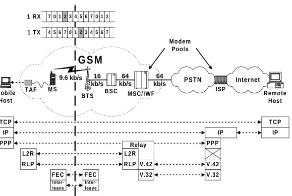
Unlike earlier analog cellular telephone systems, data services are an integral part of a GSM digital cellular telephone network and are equally supported together with ordinary voice ser-vices. Figure 2-7 shows the basic components used for circuit-switched data transmission in GSM. A mobile host, a laptop or palmtop, is connected to the GSM network using a GSM mobile phone (Mobile Station (MS)) and a device running the Terminal Adaptation Function

(TAF). Unlike in first generation analog cellular systems, the TAF is not a modem. The modem

(running the standard modem protocols V.42/V.32) resides in the network, in the Interworking

Function (IWF) of the Mobile Switching Centre (MSC). An MSC is a backbone telephone

switch that routes circuits within the GSM network and also serves as a gateway to the fixed

Public Switched Telephone Network (PSTN). The radio interface is provided by a Base Trans-ceiver Station (BTS) (or simply base station) which together with other BTSs is controlled by