A Statistical Analysis of the Aggregation of Crowdsourced Labels

(1)

A Statistical Analysis of the

Aggregation of Crowdsourced Labels

by

David Szepesvari

A thesis

presented to the University of Waterloo in fulfillment of the

thesis requirement for the degree of Master of Mathematics

in

Computer Science

Waterloo, Ontario, Canada, 2015

c

(2)

I hereby declare that I am the sole author of this thesis. This is a true copy of the thesis, including any required final revisions, as accepted by my examiners.

(3)

Abstract

Crowdsourcing, due to its inexpensive and timely nature, has become a popular method of collecting data that is difficult for computers to generate. We focus on using this method of human computation to gather labels for classification tasks, to be used for machine learning. However, data gathered this way may be of varying quality, ranging from spam to perfect. We aim to maintain the cost-effective property of crowdsourcing, while also obtaining quality results. Towards a solution, we have multiple workers label the same problem instance, aggregating the responses into one label afterwards. We study what aggregation method to use, and what guarantees we can provide on its estimates. Different crowdsourcing models call for different techniques – we outline and organize various directions taken in the literature, and focus on the Dawid-Skene model. In this setting each instance has a true label, workers are independent, and the performance of each individual is assumed to be uniform over all instances, in the sense that she has an inherent skill that governs the probability with which she labels correctly. Her skill is unknown to us. Aggregation methods aim to find the true label of each task based solely on the labels the workers reported. We measure the performance of these methods by the probability with which the estimates they output match the true label. In practice, a popular procedure is to run the EM algorithm to find estimates of the skills and labels. However, this method is not directly guaranteed to perform well in our measure. We collect and evaluate theoretical results that bound the error of various aggregation methods, including specific variants of EM. Finally, we prove a guarantee on the error suffered by the maximum likelihood estimator, the global optima of the function that EM aims to numerically optimize.

(4)

Acknowledgements

First and foremost I would like to thank my supervisor Shai Ben-David for his patience, support and the freedom he has given me in the topic of my study. I appreciate his deep understanding of many subjects, the clarity of his thoughts and communication— compelling me to work towards the same—and the feedback he provided.

I am also grateful to my parents for the example they have set for me in all aspects of life; additionally, my father for making his invaluable knowledge, insights and experience available to me in general and in the context of this work, too; my mother, as well as brother-in-law Deon and friend Shreya for the motivation, time and attention they have granted me and this project.

Finally, I would like to acknowledge my friends, in particular Neeraj, and everyone else who made my time at the University of Waterloo as pleasant as it was.

(5)

List of Tables

3.1 Comparison of the guarantees provided for various algorithms in the litera-ture.

We consider a number of algorithms with theoretical guarantees on the probability of mis-labelling; the algorithms and the bounds for them are precisely stated in Section 3.4.4. We evaluate each of these methods on the typical crowds introduced earlier, displaying the negative exponent of the resulting guarantees in this table. We useα1

.

= 1−2(1_w−ε),

(9)

List of Figures

2.1 An example of a worker label matrix, the input to the Inference Problem.

Here 5 workers (rows) provided labels for a total of 6 instances (columns) of a binary task. The entries in the matrix are the labels provided by the workers; entry (i, j) is the label assigned to instance j by workeri. If an entry is missing, the worker did not label the corresponding instance. . . 7 2.2 A possible confusion matrix.

Here “t” stands for the “true label”, “r” stands for the “response”, and the real number in entry (i, j) is the probability that the worker will assign label j to an instance with true labeli. . . 8 3.1 Confusion matrix for the one-coin model.

Here “t” stands for the “true label”, “r” stands for the “response”. p∗

i is the probability

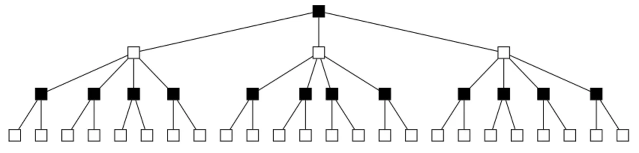
of returning the correct label, which is the same for both positive and negative labels in this model. . . 12 3.2 The locally tree-like structure of Karger et al.’s task allocation, for k = 1.

For this representation we “folded out” the bipartite graph to reveal the tree. Black vertices represent instances, white ones workers. Note, we set l = 3 and r = 5 for this illustration. . . 24 5.1 The transformed negative binary entropy acting as the Separation Criterion. 51 7.1 An illustration of the set of ε that satisfy Equation (7.1).

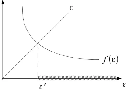
The shaded interval on the x-axis is the set of satisfying ε. We hope to find the smallest suchε,ε0, though we only do so approximately. . . 60 7.2 The contour plot of L(v, y) forw= 1 and continuous label y∈[−1,1].

Weights are shown on the horizontal axis, the continuous label on the vertical axis. For the generation of this plot the true skill was set to 2.2. . . 61

(10)

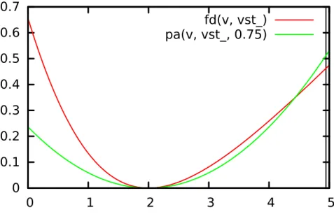
7.3 The plot of A2(v) in red andlq0.75(v) in green.

The vertical line near v= 5 isvλ forλ=

p

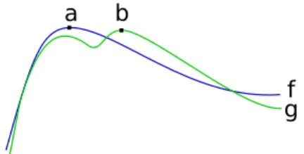
2/105_. _{. . . .} ₆₃ 7.4 Functions of bounded uniform deviation have similar maxima. . . 71 A.1 Comparing the true and approximate minimizers of fv(·, λ).

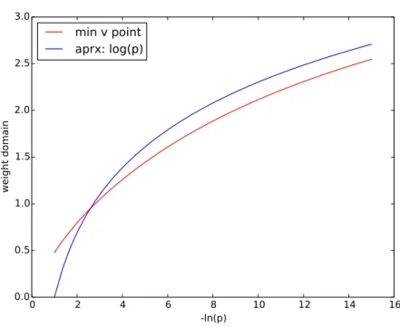
We compare, as a function of p=−log(λ), the location of the true minimizer of fv in

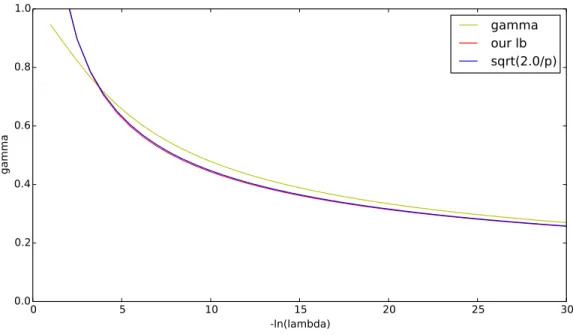
v, calculated numerically, and the approximate location used, log(p). We see that they behave similarly, with the approximate appearing to be consistently larger after some point. Note: label on the x-axis is wrong, it should bep. . . 79 A.2 The behavior of min0<v<v∗fv(v, λ).

The graph depicts 3 functions: (1) the numerically calculated bestγ∗(λ) given as min0<v<v∗fv(v, λ)

(2) our conjectured lower bound ofγ∗(λ),p2/p (3) a lower bound suggested by our anal-ysis, ₂₅1q_p₍2(_p₋p+1)_log_p₎h1− 1

2(p+1) i

(ˆv−vˇ)+p2/p. These are plotted in terms ofp=−logλ.

The graph was generated with the “find gamma approx.py” script, by running “find approx diff()” with optionsapprox="lam npow",der approx="reduced expr",value at approx estimate = np.sqrt( 2/p )anddistance estimate = (vs-v appr). . . 81 A.3 Illustrating the lower bound lγ_q with γ(p) =p2/p forv∗ ∈ {0,1,2}. . . 82

A.4 Illustrating the lower bound lγ_q with γ(p) =p2/p forv∗ ∈ {3,4,5}. . . 83

A.5 Illustrating the lower bound l_qγ with γ(p) = p2/p for v∗ = 6 at the same

(11)

Chapter 1 Introduction

Crowdsourcing, a recent buzzword, refers to the process of distributing jobs to a large group of people over the internet. The so-called workers get exposed to more opportunities through which they can earn a wage, and for the employers it provides a convenient, quick, and often cheap way of getting tasks done that would otherwise require hiring someone. Nonetheless, crowdsourcing is not always monetarily motivated; the Zooniverse1 _{project is}

one of the numerous “volunteer research” platforms.

Our main motivation of using crowdsourcing is to collect labels for supervised learning. In modern-day techniques, predictors get trained on thousands, if not millions of examples. With crowdsourcing these labels can often be collected in a cheap and timely fashion; the caveat being that the quality of these labels is not guaranteed and in fact, a large part of it can even be spam. One solution is to request multiple workers to solve, or in our case label each problem. For many crowdsourcing problems, identifying the best solutions can be done manually. However, given the large quantity of data we are considering, there is a need for an automated method. We aim to aggregate responses, from a number of sources of varying reliability, into labels for each supervised learning instance that we believe are perfect with high confidence.

This is a popular and well-studied problem. We devote the next chapter to outlining and organizing a number of approaches taken in the literature. In the remainder of the thesis, we focus on the theoretical aspect of the problem, that is, we wish to see and provide guarantees on the performance of various aggregation methods. Moreover, we want these guarantees to come in the form of a mislabelling error: assuming that each problem to be labelled has a true label associated to it, we wish to obtain that label with high probability.

(12)

We select the one-coin model (an instance of the Dawid-Skene model) — which is simple, yet effective — and discuss in-depth the available knowledge pertaining to it. The key assumption in this model is that each worker providing labels has an inherent level of reliability that is uniform over her labelling, governing the probability with which her labels are correct. In order to better reflect on the performance of aggregation methods used and analysed in this setting we use a tabular representation, contrasting the guarantees offered for each, in various stylized scenarios.

In the model of our choice, one of the most common practical aggregation algorithms is the well known EM meta-algorithm. As EM is not directly guaranteed to perform well according to our natural measure, there have been various studies to establish the low mislabelling error (Gao and Zhou, 2013; Zhang et al., 2014). We uncover an important mistake in a proof given by Gao et al.Gao and Zhou(2013) pertaining to the performance of the global maximizer of the function EM optimizes. Furthermore, we set out to prove an upper bound in a similar setting. To be precise, we consider the maximum likelihood estimate and work towards a proof of an upper bound on its probability of mislabelling. We finish with a finite sample bound that controls the error rate of these estimates, but relies on a simple analytic statement that is well-justified, albeit not yet proven.

Outline. In Chapter 2, we detail the crowdsourcing scenario considered along with the common problems related to it. Chapter Chapter 3 specifies the model we work with in full mathematical detail while introducing some notation used throughout the thesis. We also quote and discuss relevant statements from the literature, and present their guarantees for an overview. Chapter 4 elaborates common techniques that will be used in the proofs towards the main result. Finally, Chapter5shows our main results leading up to a bound on the error rate of the maximum likelihood estimates. In Chapter 6, we conclude the thesis, reflecting on our result, its place in the literature, and outlining directions in which the investigation could and should continue. Chapter 7 holds the proofs of the mathematical claims made throughout the thesis.

(13)

Chapter 2 Crowdsourcing Problems

Our motivation is to collect labelled examples for (semi-)supervised learning. Historically there was a shift from supervised to semi-supervised learning motivated by the fact that in many domains unlabelled data is abundant, does aid learning, and labels are costly in comparison. With crowdsourcing, however, one now has access to cheap labelled data – though of possibly low quality. The goal is to have the cake and eat it too; can we boost the quality of the labels acquired from crowds while keeping the cost low?

In order to boost the label quality, we ask multiple workers – who are assumed to be labelling independently of each other – to label the same instance. We can report the majority label as our estimate with increased confidence. Clearly, then, a strategy is to keep adding such independent workers. However, we would like to keep costs as low as possible, therefore study whether there are more “efficient” ways to combine, oraggregate

the labels provided by the workers. We will make the key assumption that the performance of each worker is in some way consistent over all instances of a task. Details vary between different works, but in general the inclusion of this assumption does enable significant improvements over the above mentioned majority voting in the label quality-cost trade-off. For an illustration, consider the situation that there are some instances of the problem where all the workers specified the same label. This increases our confidence in these workers’ abilities, and we trust them more than others. This, in turn, may reveal that there are other instances where workers appearing skilful are mostly in agreement. Again, we use this information to adjust our evaluation of the workers. Eventually, we get a sense of the workers’ skill, while providing estimates for the labels that takes this into account. Although the pattern exploited in this illustration may be more subtle in typical data gathered through crowd-sourcing, it is still possible to utilize it.

(14)

Note that this process of gathering labels of unknown quality is not exclusive to crowd-sourcing. The sources of the labels are irrelevant, as long as it is sensible to make the required assumptions. An important example is the aggregation of labels from already trained classifiers. The problem of aggregating classifiers is well studied in statistical learning, though traditionally this is done using labelled data. The crowdsourcing problem may be interpreted as the aggregation of classifiers using unlabelled data; the recent work ofJaffe et al. (2015) is, in fact, phrased in such a way.

This chapter presents the general framework we consider and provides an overview of the research studying it. We describe a typical crowdsourcing platform, as well as the nature of the data collected with it. We then identify three problem families dealing with crowdsourced data. Independently of these, we categorize works based on the relationship they assume between the labels to be recovered and those provided by workers.

2.1 The Nature of Crowdsourced Data

Since our study is motivated by the use of crowdsourcing to acquire labels for machine learning tasks, in particular classification, we often require a copious number of instances to be labelled by the crowd, with each individual instance quickly categorized by a human in exchange for a small sum of money on the scale of 1-3 cents. Such crowdsourcing tasks are often referred to as microtasks. We outline here key facts about Amazon Turk (Amazon, 2015), a crowdsourcing site, which was the first well-known such platform and is still popular in the microtasking community. Its system is representative of a large body of crowdsourcing sites:

• It is the workers that decide which tasks they will do. That is, employers cannot request workers, let alone workers of given accuracy. However there are ways – widely used in the hope of reducing the amount of spam – to filter the workers that can even attempt the task based on a simplistic system-wide measure of reported reliability. This does not actually seem to stop spammers, however (Ipeirotis, 2010).

• It is possible to require training of workers before they can attempt a task.

• It is possible to reject work submitted by a worker, meaning they will not be paid. This should not be done lightly, though, as it may result in a bad reputation of the employer, with workers not even attempting future tasks (Chen,2012;Kumar,2014).

(15)

• It is reasonable to require workers complete some given number of instances per payout. However, more often each payout is tied to a small number of instances with the system making it simple to continue with new instances of the same task. In fact, workers tend to grind on one task if they like it. This means we can mostly expect two types of workers: ones who complete a few tasks, and ones who do many –measured in 10s, 100s or even 1000s (Chen, 2012; Kumar,2014; redditer,2014). • Each user’s ID is available with their submission, so they can be identified.

• It is possible to specify that workers cannot repeat the same instance multiple times. Note that the last bullet point aids in actually enforcing the assumption that sources are independent. Furthermore, that the fact that IDs are available with each submission allows us to identify and track each worker, which is needed in order to utilize the assumption on the workers’ labelling performance. On the other hand, it is apparent that controlling the quality of responses is difficult; it is expected to see spammers whose responses carry no information about the true label of the instances. Workers exerting effort may also make varying numbers of mistakes.

The Amazon Turk framework has a serious limitation: it is not possible to request specific workers. Put differently, workers cannot be allocated to specific tasks or even instances. This would likely increase the efficiency of a smart microtasking and label aggregation system – though it also brings up various design questions. We concentrate on the system offered by Amazon Turk and other similar platforms, as it is the most widespread contemporary design.

A word on label quality: It is important to note that in practice the way labelling

problems are presented to the worker have a tremendous effect on the quality of each individual worker label. While not the prime example of a microtask, in a Zooniverse task (Zooniverse, 2015) involving labelling animals on pictures taken by deployed cameras in the Serengeti, the user interface helps with identifying the type of animal. This is based on a number of features that individually become simple labelling tasks (e.g. the shape of the horn of the animal, if any) and act as filters on all possible answers to the original instance. In effect, the daunting task is broken down into a sequence of easily manageable problems. Similarly, even attributes of the batch of instances submitted to a crowdsourcing system, such as the number of total available tasks, the default payment delay and the payout also influence the quantity and the quality of the labels from the workers (Kumar, 2014; Chen, 2012). While it may be interesting to study how to motivate or optimize for quality labels, it is not our focus. We take the labels received granted, and aim to aggregate them effectively.

(16)

2.2 Mathematical Formulations of Label Aggregation

There are various directions in studying label aggregation; we characterize them in two independent ways. We first describe a range of aggregation problems with increasing degree of freedom, then we categorize works by how they model the relationship between the true and worker labels. First, however, let us establish a common dictionary, and with it a precise statement of the scenario investigated.

Setup. In the crowdsourcing setting we have instances of tasks, each with its own (true) label. These labels, however, are generally not known to us, and we askworkers orlabellers

to label them. We see the labels they provide, and refer to these as worker labels. The workers are assumed to have an inherentskill that, vaguely speaking, captures how good they are at labelling instances of tasks. A task here refers to a type of labelling problem, containing many instances that are homogeneous in nature. We may speak of multiple tasks to express that the skill of a worker on one task may be different from her skill on another task. Unfortunately the term task difficulty, which should really be instance

difficulty, corresponds to varying levels of labelling hardness amongst otherwise similar

instances, even for the same worker. The reason for this terminology is that in the literature concerned solely with homogeneous instances each instance is, in fact, often referred to as a task. As the main focus of this thesis is the homogeneous setting, we will also adopt this convention starting in the next chapter. Until then we maintain the distinction for clarity. All instances are uploaded to a crowdsourcing system byemployers orrequesters. Requesters may use gold(en) units, also known as gold standards, instances whose true label they know – these can be used to test workers. Finally, variables such as skills, task difficulties and sometimes the true labels as well, are often referred to asparameters.

Our goal is to recover the true label of each instance. We quantify the success of various methods as the fraction of instances whose label they recovered correctly. In the context of the statistical models used in the literature, we may say weinfer orestimate the true labels. When analysing inference methods in this setting theoretically, our measure of success translates into the expected value of the fraction of mistakes made, or more generally the cumulative distribution of the same (random) quantity.

2.2.1 Categorization by Degrees of Freedom

(17)

      + − + + − + − + − + − − − + + + − − + + + −      

Figure 2.1: An example of a worker label matrix, the input to the Inference Problem. Here 5 workers (rows) provided labels for a total of 6 instances (columns) of a binary task. The entries in the matrix are the labels provided by the workers; entry (i, j) is the label assigned to instancej by worker

i. If an entry is missing, the worker did not label the corresponding instance.

• Prediction Problem: given the parameters (other than the true labels), upon observ-ing labels for a new instance output an estimate for its true label. More generally, we may only have estimates of the parameters (Berend and Kontorovich, 2014). • Inference Problem: upon seeing only the labels provided by the workers on a number

of instances, infer the true task labels, possibly other parameters as well. The input to the inference algorithm can be thought of as an incomplete matrix that collects the responses from the workers; see Figure2.1for an example. Additionally, the methods may incorporate golden data as well, though the key is that they effectively utilise the worker labels arriving from dubious sources in the estimation of the true label. As outlined above, we measure performance by the portion of true labels recovered. This is the classical crowdsourcing aggregation problem, with works including that of Whitehill et al. (2009); Welinder et al. (2010); Liu et al. (2012); Gao and Zhou (2013); Zhang et al.(2014); Jaffe et al.(2015) and this thesis.

• Instance Allocation: (interactively) allocate instances to workers in order to infer the true task labels (and other parameters) with as few queries as possible (Kolobov et al., 2013; Bragg et al., 2014; Abbasi-Yadkori et al.,2015).

The main results inKarger et al.(2011b,2013,2014) fix a specific allocation before seeing any labels, and solve the inference problem once the labels do arrive; this places them closer to the second category.

There are also various other directions studied that are outside the scope of this doc-ument; we highlight two here that are more closely related to our interests, though. Liu et al.(2015) consider the inference problem, but insert gold units after the data was col-lected, one by one, in order to try to get the best increase in label quality. A line of work in task allocation (Ho et al.,2013;Jung,2014) considers allocating different tasks to workers,

(18)

t\r - + - 0.8 0.2 + 0.3 0.7

Figure 2.2: A possible confusion matrix.

Here “t” stands for the “true label”, “r” stands for the “response”, and the real number in entry (i, j) is the probability that the worker will assign label j to an instance with true labeli.

not simply instances. They aim to automatically find similar instances and utilize this information in the allocation methods.

2.2.2 Models of Labelling

Some sort of model describing the relationship between the true and the worker label is required for any result. Most papers in this domain explicitly work with a simple expression for the probability of a worker mislabelling an instance. We may phrase many such popular models in either the Dawid-Skene or the Joint CrowdSourcing (JoCR) model. We now describe these in detail, mentioning their variants that appear in the literature. Afterwards, some models that work under significantly different assumptions are also mentioned.

Dawid-Skene model. This model was introduced by Dawid and Skene in 1979 (Dawid et al., 1979) and has become a classical label crowdsourcing model forming the basis for a fruitful line of research (Karger et al., 2011b; Liu et al., 2012; Li et al., 2013; Berend and Kontorovich,2014), recently culminating in methods claiming (near-)optimal results (Gao and Zhou, 2013;Karger et al.,2014; Zhang et al.,2014). Most work is set in the Inference Problem scenario.

We assume each worker has a latent confusion matrix describing the joint probability distribution over true and reported labels. An example of such a confusion matrix for the case of binary classification is shown in Figure2.2. The worker with the confusion matrix shown on this figure will label negative instances correctly with probability 0.8, positive instances with 0.7. Other workers may have completely different confusion matrices.

Considerable amount of research is focused on labelling binary tasks; then the model is also referred to as the two-coin model. We may further specialize it by restricting the diagonal entries to be equal. This model is called the one-coin, or sometimes the Symmetric Dawid-Skene model. It models uniform behaviour over the two classes, and hence we lose the ability to model worker bias.

(19)

Joint CrowdSourcing (JoCR). The general JoCR framework was introduced byKolobov et al.(2013). The main merit of JoCR is that it is able to model a possibly ever-changing pool of workers, allocating tasks to them in real time. Note that some of the work refer-enced in this category works only on a static pool, though, or was published outside of the JoCR framework but can be naturally rephrased in its notation.

There is a set of tasks Q, each task q ∈Qwith a small number of possible answers Aq.

Each task q has an inherent difficulty dq, and each worker w ∈ W has an inherent skill

γw, where W is a pool of workers, which may or may not be changing from timestep to

timestep.

The probability that worker w will label question q correctly is p(dq, γw), that is, it

depends only on these two parameters. Note that this assumption, again, implies we cannot model bias towards certain labels. Different functions p may appear in different works, however, we often can re-parametrise one into the other. We present some examples that model truly different assumptions.

• The model that appeared most prominently, for example in the work of Bragg et al. (2014), is p(dq, γw) = 1 2 h 1 + (1−dq) 1 γw i ,

where dq ∈[0,1] and γw ∈(0,∞). Note that this assumption cannot model workers

who tend to label incorrectly.

• For anonymous workers the model reduces to _P(correct label for j) = diffj, that is,

we only have difficulties. HereAbbasi-Yadkori et al.(2015) is interested in optimizing the order in which the instances of unknown difficulty should be put up for labelling. • The model used by Whitehill et al. (2009) for inference also falls into this category:

p(dq, γw) =

1 1 +e−dqγw.

Here the probability of worker w labelling an instance with difficulty dq correctly is

modelled by the logistic function with input −dqγw for γw ∈ [−∞,+∞] and dq ∈

[0,∞]. This functionp generalizes the one-coin model by introducing difficulties. We illustrate the existence of models that do not explicitly work with the probability of labelling correctly, rather they describe the process as a sequence of steps. Welinder et al. (2010), for example, describe:

(20)

1. Each instance is mapped to a vector characterization that correspond to features a perfect labeller would consider in order to label the instance. This step can capture some instances being more difficult than others.

2. Each individual worker observes these features with varying degrees of accuracy. This is modelled by using a gaussian noise of different variances on the different features, according to the skill of the worker.

3. The worker reports a label based on their internal affine decision boundary. They explicitly incorporate biases, and model different levels of uncertainty quite well.

(21)

Chapter 3 Inference in the Dawid-Skene Model

We work in a special case of the Dawid-Skene model. Nonetheless, we first precisely introduce the model in its generality, then restrict our attention to its simplification. This will clarify the relationship between our and the general model, and will also allow us to discuss results more effectively. Though we have already outlined and provided context for the inference problem and the Dawid-Skene model, this chapter is devoted to the detailed and mathematically precise treatment of these topics, followed by an in-depth investigation of the theoretical literature on crowdsourcing in this setting.

3.1 Problem Definition

We follow a number of conventions. First, matrices and random variables will be denoted by capital letters unless otherwise specified. Vectors and scalars most often are lower case. We use the notation [n] = {1,2, . . . , n}, and _I{·} for the indicator function. The model will include a number of parameters, and these will be estimated. Generally the true parameters receive a star, as in p∗_i or p∗, estimates a hat ˆpi. Note that these estimates

are truly the output of estimators on the random data, and, as such, random variables. Arguments to functions playing roles similar to these parameters will stand without any decoration. We use 1 to denote vectors whose components are all one. All vectors are column vectors unless otherwise noted. We use ·> _{to denote the transpose operation.}

Finally, we note that log denotes the natural logarithm.

General Dawid-Skene. There aret -for task- instances of a K-way classification task, with instances commonly indexed by j. Here we assume the labels are from the set [K].

(22)

t\r - + - p∗_i 1−p∗_i

+ 1−p∗_i p∗_i

Figure 3.1: Confusion matrix for the one-coin model.

Here “t” stands for the “true label”, “r” stands for the “response”. p∗_i is the probability of returning the correct label, which is the same for both positive and negative labels in this model.

Each instance j has a true label y∗_j ∈[K], collectively denoted by y∗ ∈ [K]t. There are w

workers, indexed by i, each with an inherent confusion matrix P_i∗ = (p∗_i,cl)c,l ∈ [0,1] K×K

,

p∗_i,cl holding the probability that worker i labels an instance with true label c as l. That is, we must haveP

l∈[K]p

∗

i,cl = 1 for any c∈[K]. Here we assume that every worker labels

every instance, though it is common to model missing values by assuming that whether a worker labels a task is like a Bernoulli random variable with some parameter specific to that worker. The worker responses may be formatted into a matrix. We denote the random variable corresponding to the reported label of worker ion instance j by Yij, and

the random matrix that collects these by Y. The Dawid-Skene assumption, then, can be written as

P(Yij =l) =p∗i,y_j∗l, i∈[w], j ∈[t], l ∈[K] and

(Yuv)(u,v)∈A ⊥(Yxy)(x,y)∈B for A, B ⊂[w]×[t], A∩B =∅,

where the second line records that theYij are mutually independent.

One-coin model. As mentioned earlier, the one-coin model is the special case of the Dawid-Skene model where we only consider binary tasks, and assume that workers exhibit no bias toward either class. The simpler notation we introduce here is what the rest of the thesis will use.

In this case we redefine the labels to be either positive or negative, that is, y∗ ∈ {±1}t.

Due to the additional assumption on the confusion matrix, we now have just one parameter

pi ∈[0,1] determining the whole confusion matrix shown on Figure3.1. Formally, for any

worker i

p∗_i,cl = (

p∗_i , c=l; 1−p∗_i , c6=l,

that is, workers label correctly with probabilitypi. Instead of working withp, we introduce

(23)

s indicates whether the worker is biased towards the correct label, or they are more likely reporting the wrong answer. The magnitude ofs, in turn, clearly communicates how strong the worker’s bias is. In particular, ifs= 0, we have a spammer; if |s|= 1, then our worker is what we call perfect - though may be malicious. Again, the individual worker skills s∗_i

form the vectors∗. With this, the one-coin model assumption can be written as

P Yij =yj∗ = 1 +s ∗ i 2 , for i∈[w], j ∈[t] and (Yuv)(u,v)∈A ⊥(Yxy)(x,y)∈B for A, B ⊂[w]×[t], A∩B =∅.

(3.1)

Finally, it will be convenient to work with the random variable Tij denoting whether

the reported worker label for a given task is correct. Define

Tij

.

= 2_IYij =y∗j −1∈ {±1}.

Convenient alternative ways to write this are

Tij =y∗jYij, Yij =yj∗Tij.

Note that, Tij ∼2 Ber ₁₊_s∗

i

2

−1, and therefore _E[Tij] =s∗i.

The goal. Our main focus is the inference problem: upon observing the labels provided by the workers we wish to find y∗.

More precisely, we wish to find an estimation “procedure”, A:{±1}w×t_{→ {±1}}t _that

achieves low loss, measured as the probability of mislabelling a uniformly randomly chosen taskJ:

`(A)=. _P(A(Y)J 6=yJ∗).

The loss of a procedureAwill depend on the input distribution; which is fully characterized by the skillss∗ of the workers and the true labelsy∗ of the tasks. Naturally, we wish to find

a procedure that has low loss for all possible input distributions. To enable this discussion, we make explicit this dependence: denote by `(A,(s∗, y∗)) the expected loss of procedure

A when run on data conforming to the Dawid-Skene model with parameters (s∗, y∗). We,

not unreasonably, ask that a procedure A achieve small loss over any true label setting, that is, we measure its performance as

sup

y∗∈{±1}t

(24)

On the other hand, it is also reasonable to expect that procedures are able to perform better when the workers are generally more qualified. In order to capture this, we may wish to compare the performance of A to so-called oracles that are aware of the skill of each worker. The loss associated to the best oracle is captured by

`∗(s∗)= inf.

A _y∗_∈{sup_pm₁_}t

`(A,(s∗, y∗)), (3.3)

where the infimum is over the procedures. Indeed, since s∗ is fixed, the best choice

for A in this expression can depend on s∗. We will see in Section 3.4 the optimal

or-acle rule and a tight characterization of the loss it suffers. Observe that comparing infAsupy∗∈{±1}t`(A,(s∗, y∗)) to`

∗₍_s

∗) reveals the additional difficulty of the inference

prob-lem introduced by the unknown skills.

Additional notes. There is an inherent ambiguity in this model. Consider the true generating parameters (s∗, y∗) and their negation (−s∗,−y∗), meaning the workers have

the same absolute skill but report the opposite answer, and the generating true label also flipped. These are impossible to distinguish based on the observed worker labels. To break this symmetry we assume

X

i

s∗_i >0, (3.4)

that is, on average, the workers are biased towards the correct answer. For the purposes of the analysis we will evaluate our procedures against both the true and flipped labels, and take the better, that is,

`(A) = min{_P(A(Y)J 6=yJ∗),P(−A(Y)J 6=yJ∗)}. (3.5)

Eventually we will investigate under what conditions, in addition to Equation (3.4), we are able to differentiate between the two otherwise symmetric label assignments. The final note to make is that for the purpose of the analysis and without loss of generality, we assume that y∗ =1. This indeed can be done as long as the estimation method A is not

biased towards any label.

3.2 Discussion of the Model

As any result stated is only guaranteed to hold when the data matches our model, it is important to evaluate how realistic the model is. On the other hand, one should not

(25)

mistaken the conditions as to being necessary for algorithms to work. In fact, it is very likely that the algorithm can produce good results under weaker conditions, too.

With this in mind, let us discuss the constraints imposed by the model. The inde-pendent source (worker) assumption may be violated for a number of reasons. Clearly, if workers copy or simply collaborate they cease to be independent. However, for microtask-ing problems where each individual instance takes only seconds, with a platform such as Amazon Turk where it is not possible to transfer answers to a large number of instances, this is not likely to be an issue. We also suppose that the performance of the worker is uniform over all instances. This is quite possibly not true, even when the instances are ho-mogeneous in nature. However, experimental work suggests that despite this, such models still lead to significantly better results than the baseline majority voting.

Altogether the model imposes a rigid structure on the labelling process, and, as shown byGao and Zhou(2013), can lead to performance worse than uniform majority in misspec-ified models: consider two types of tasks and two groups of workers. The first group labels very well on task type I, and knows nothing of type II, and vice versa. If the two worker groups are equal in size, the number of the instances belonging to each task is imbalanced in a quadratic fashion, and the number of tasks is significantly larger than the number of workers, assuming the Dawid-Skene model and the maximum likelihood estimates suffers loss (measured in expected average number of mistakes made) that converges to zero at a rate only polynomial in the number of instances. In contrast, the error rate of majority voting still converges exponentially fast in the number of workers. Note that while these are stated in terms of different parameters, the above statement about the convergence rate in the Dawid-Skene model implies that it is also polynomial in the number of workers. While an important illustration, the setup used is not typical of simple, homogeneous la-belling problems – for these the one-coin model, or more generally the Dawid-Skene model is reasonable, and this is supported by the large number of experimental work showing the benefits of these models in practice.

One final technical assumption made is that every worker labels every instance. This can be relaxed; for instanceZhang et al.(2014) introduce a “labelling probability” specific to each worker in addition to their skills. This is a good model when the worker does not choose to skip instances, and the order in which she was presented with them was chosen uniformly randomly from all orders.

(26)

3.3 Performance Baselines

Before presenting results from the literature, we prepare by specifying a number of ways in which they can be evaluated. The first method to consider for the aggregation of the worker labels is (Uniform) Majority Voting (MV): the algorithm that outputs the label that was reported the most often, individually on each task. Note that MV is indifferent to the skills of the workers, therefore one hopes that inference methods that do take skills into account will outperform it. An upper bound on the loss of MV is presented in Section 3.3.1. Afterwards, in Section 3.3.2, we define various stylized types of crowds, or worker collections, on which we evaluate the error bounds associated to the inference methods in the literature. These error rates will be compiled into a table, namely 3.1, at the end of the chapter.

3.3.1 Majority Voting

Uniform Majority Voting is a special instance of the weighted majority voting (WMV) algorithm. We define, forv ∈_Rw_{, the} _v_{-weighted majority rule to be}

f_vmaj:{±1}w → {±1}

x 7→sgn x>v, (3.6)

wherexserves as the collection of worker labels on an instance. Note that the scale of the weight vector has no bearing on the decision rule, that isf_vmaj =f_rvmaj for all r >0. While the case that x>v = 0 is not handled by the definition, we will turn a blind eye, and for the purposes of the analysis we will assume this results in an error. We can extendfmaj

v to

allow weights that have components infinite in magnitude, but only if all such components have the same sign. Finally, by abusing notation, we shall also writef_vmaj for the extension of this map to a {±1}w×t _{→ {±1}}t _{map, where} _fmaj

v (Y)j

.

= fmaj

v (Y:j), 1 ≤ j ≤ t and Y:j

stands for the vector (Yij)1≤i≤w, i.e., the jth column of Y.

Uniform Majority Voting (or simply Majority Voting) is WMV with uniform weights – for instance v = 1, – and will be denoted by fmaj_{. We see that this indeed reduces to} reporting the label that occurred more often. In Section5.2.1 (Corollary 2) we show that for a task with true labely∗,

P fmaj(Y)6=y∗ ≤exp −1 4 Xw i=1 s∗_i v∗_i −1Xw i=1 s∗_i 2! (3.7)

(27)

holds, wherev∗_i denotes the log-odds of worker i labelling correctly, that is,

v_i∗ = log1 +s

∗

i

1−s∗_i. (3.8)

We will later see that the star notation, suggesting –by our convention– that these are “true” weights is in a sense justified. The expression in the exponent of the bound is somewhat convoluted. We offer two simplifications. For the degenerate case of every worker having the same skills∗_i =s∗₀, the exponent becomes −1

4s ∗ 0v ∗ 0, where v ∗ 0 = log 1+s∗ 0 1−s∗₀.

We will see the same (up to a constant) in Section 3.4.1, where it characterises the error of the optimal decision rule. The coincidence is only under this uniformity assumption. Alternatively, we notes∗_i/v∗_i =s∗_i/log 1+s∗i

1−s∗

i ≤1/2 no matter the value ofs

∗ i ∈[−1,1], which leads to P fmaj(Y)6=y∗ ≤exp −1 2w 1 w w X i=1 s∗_i 2! . (3.9)

This is really loose; we have s∗_i/v∗_i → 0 as |s∗_i| → 1, yet we upper bound it by 1/2. On the other hand, to the best of our knowledge, this was the bound known for the error of majority voting before; for exampleLi et al. (2013), in their Corollary 6, offer the same.

3.3.2 Stylized Crowds

We define some special, parametrized collections of workers that will help reveal the be-haviour of the bounds proved on the various inference methods. The first two are well-known in the literature, and are commonly used for lower bound arguments; the third is our addition as far as we know. There are three measures of crowds that commonly appear in bounds: the average of the skills (¯s), the average of the absolute values of the skills (¯µ), and the average of the squares of the skills (¯ν). We show each of these for every crowd considered.

Uniform. Perhaps the simplest crowd: let each of the w workers have the same skill s. A crowd with this property will be referred to as CU

s . The associated measures are ¯s =s,

¯

µ=|s|, and ¯ν =s2_.

Spammer-hammer. Everyone in our crowd either has s = 0, a spammer, or s = 1, called a hammer. Such crowds demand that inference algorithms be able to differentiate between workers of vastly different skills. This class,CSH

q , is parametrized byq, the portion

(28)

Evil Twins. Out of 2w + 2 workers w has skill 1, w has skill −1, and 2 have skills

ε >0. This crowd is very knowledgeable, therefore we can expect near perfect labels from inference methods able to differentiate between malicious and honest workers. We useCET

ε

to refer to this type of crowd, parametrized by the bias of the near-spammer workers. In this case ¯s= 2ε, ¯µ= 1− 2(1_w−ε), and ¯ν = 1− 2(1−_wε2).

3.4 Existing Results

We collect, under a unified notation, and discuss the existing theoretical knowledge per-taining to the inference problem in the Dawid-Skene and the one-coin model. This work spans the past years, recently culminating in results claiming (near)-optimality. It has been long known (Nitzan and Paroush, 1982) that weighted majority voting with weights corresponding to the log-odds of the worker labelling correctly leads to optimal decisions. That is, the optimal decision rulefOPT _{is given by} _fmaj

v∗ : sgn x>v∗ = sgn   X i∈[w] xilog 1 +s∗_i 1−s∗ i   , (3.10)

forx= (xi)i ∈ {±1}w,s∗ ∈[−1,1]w. The rule is optimal in the sense that it has loss `∗(s∗)

(cf. Equation (3.3)); this can be derived from the Neyman-Pearson lemma. However, until recently it was not clear what error this method suffers. Berend and Kontorovich (2014) show an improved upper bound on the probability of mislabelling, as well as an asymptotically matching lower bound. Details of these and additional results can be found in Section3.4.1. Li et al.(2013) explored the error rate for all hyperplane rules, considering missing worker labels as well. When skills are unknown the problem becomes considerably harder.

Karger et al. (2011b,a), in a sequence of works, proposes various methods to estimate binary labels in the one-coin model, finally achieving minimax optimality in some measure; although, they require a special structure on the allocation of instances to workers. They first notice that the worker response matrix has low-rank with the first left and right singular vectors corresponding to true labels and skills, respectively. Later they replace this estimation method with an almost identical message-passing algorithm for which they can show much stronger, exponential bounds on the error rate. This analysis relies on having a very large number of tasks and workers, however. Details are deferred to Section 3.4.2.

Ghosh et al. (2011), also working in the one-coin model but with (nearly-)full worker response matrices, applies singular value decomposition toY Y> to obtain bounds similar

(29)

to that of Karger et al. (2011b). Dalvi et al. (2013) analyse any allocation in terms of the so-called expansion gap of the bipartite graph on instances and workers induced by the labelling. They show finite sample bounds on the error of the skill estimates measured in squared `2 norm, which in the special task allocation of Karger et al. (2011b) leads to an exponential bound on the expected number of mistakes. Jaffe et al.(2015), working in the two-coin model, use spectral methods on the same matrix as Ghosh et al. (2011) do and show asymptotic rates on the recovery of the confusion matrix.

Another approach taken by Gao and Zhou (2013); Zhang et al. (2014) is the analysis of a regularized log-likelihood function associated to this model, and the EM algorithm that attempts to find its maximizing parameters: the generating skills and true labels. The log-likelihood function corresponding to this model is not convex, therefore EM is not guaranteed to find maximum likelihood (ML) estimates. Moreover, the ML estimate of a model does not automatically enjoy low loss. In a paper only published on arXiv (though cited a number of times) Gao and Zhou (2013) claims a minimax optimal exponential bound on the loss for both the global maximizer of the regularized log-likelihood function and the estimate returned by a slightly modified version of EM. We have found a mistake in the proof of the former and communicated it to the authors – who have confirmed it, while the argument for the latter bound stands. In fact,Zhang et al. (2014) use the same analysis of the same modified EM algorithm, now in the multiclass and fully general Dawid-Skene setting, to claim near-optimal sufficient conditions for a perfect label reconstruction. For EM to be successful with high probability, a special, spectral-based initialization is used. Details appear in Section 3.4.3. The bound we prove in Chapter 5 is on the global maximizing parameters of the likelihood function for the one-coin model. As such, we fill the gap that opened in (Gao and Zhou,2013); though, our bound is presented in a different form.

Chapter 4 introduces a number of topics, including the log-likelihood function, EM and concentration inequalities familiarity with which may be needed for the more in-depth discussions in the following sections.

3.4.1 Known or Approximate Parameters

We start with studying the simpler case when the skills are known, or we are given estimates of them, and only the true labels remain to be inferred. The resulting rates serve as a benchmark, and also reveal quantities that characterize the effectiveness of a crowd of workers. The definitive work on this topic is that ofBerend and Kontorovich(2014). They work in the one-coin model, and are concerned with the error made by the optimal decision

(30)

rule,fOPT _:_{±1}t _{→ {±1}, given by Equation (3.10). It is shown that the so called}_(total) committee potential Φ = X i∈[w] s∗_i log1 +s ∗ i 1−s∗_i (3.11)

governs the probability of making an error. For a single task (i.e.,t = 1) we have

P fOPT(Y)6=y∗ ≤exp− 1 2Φ , (3.12) P fOPT(Y)6=y∗ ≥ 3 4[1 + exp(2 Φ + 4√Φ)]. (3.13) In short, we see that

−log_P fOPT(Y)6=y∗

Φ,

where denotes equivalence up to universal multiplicative constants. Both the lower and upper bounds are contributions of this paper. The upper bound is proven using Kearns and Saul’s inequality (Lemma3), which is tighter in this setting than other commonly used concentration bounds, and is therefore of interest to us as well. Note that the committee potential increases with each additional (non-spammer) worker; sometimes we may wish to talk about the average committee potential, _w1 P

i∈[w]s

∗

iv∗i, denoted by Φ, instead. This

notion is especially informative when analysing the effects of the quality of the crowd and the number of workers separately.

In addition to the known-skill setting, the scenario where the skills are estimated on a number of golden units, instances with known labels, is also studied, both from a frequentist and a Bayesian point of view. In the frequentist approach, one option is to replace the true skills in the weighted majority decision rule by the estimates ˆs ∈[−1,1]w_{, yielding weights}

ˆ

vi = log1+ˆ₁₋_si_ˆsi and the rule fˆvmaj. We base the proof of our Lemma 11 on the argument of

Berend and Kontorovich who showed a finite sample bound on the mislabelling probability of f_ˆ_vmaj. The form of their bound is as follows. For any 0 < δ < 1, 0 < ε < min{5,2Φ}, letting ti denote the number of golden units worker i was tested on, if

ti(1− |si|)≥6 √ 4ε+ 1−1 4 −2 log 4w δ , then P f_ˆ_vmaj(Y)6=y∗ ≤δ+ exp −w(2Φ−ε) 2 8Φ .

Hereδ is associated to the probability of receiving a non-representative sample of worker labels on the golden units,εcaptures how much we err when estimating weights. Note that

(31)

the bound captures the additional error suffered over that of the optimal oracle decision rule due to having to estimate the skills.

3.4.2 Inference with Task Allocation

In this section we discuss inference results that require a special instance, or worker-task pairing. This allocation of worker-tasks to workers, however, is designed statically before any labelling takes place, the workers then provide their labels on the tasks that were assigned to them, and finally an algorithm aggregates these into estimates of the true labels. Karger et al. (2011b,a, 2013, 2014) design inference methods in this setting. The results that they derive have since been superseded by other works, which do not even require such specific assumptions on the structure of labelling. Nonetheless, it is educational to examine the methods they propose as well, for they provide a different perspective on the same problem. Moreover, while not our current focus, these works also allude to adaptive (dynamic) task allocation. Karger et al.(2011b) characterize their crowd by the quantity ¯ ν= _w1 P i∈[w](s ∗ i)2 = w1 ks∗k 2

2, and show upper and lower bounds (for relatively weak crowds) on the mislabelling probability of their methods in the one-coin model, with ¯ν appearing in the exponent of both. Another important quantity they work with is the number of times each task is labelled, l, in their task-allocation. This is considered to be small; in fact their final results are phrased in the form of bounds onl when other problem parameters, including the probability of mislabelling, are fixed. The first paper (Karger et al., 2011b) introduces the instance allocation procedure, and uses singular value decomposition on the collected worker labels to recover the skills and true labels. The resulting upper bound on the loss ` (cf. Equation (3.2)) is only in the order of _l1_ν_¯. The following paper (Karger et al.,2011a) replaces the inference method by a message passing algorithm that is almost identical, but allows for an analysis leading to a bound on the loss that is now on the scale of exp(−lν¯). A significantly extended version of the same conference paper was published some time later (Karger et al., 2014). Finally, Karger et al.(2013) reduce the multi-class, general Dawid-Skene problem to a number of binary tasks, for which they call their already proposed estimation, yielding a near minimax optimal algorithm.

Instance allocation. Intuitively, the instance allocation proposed aims to spread the workers out evenly over the instances. An allocation will be represented by a bipartite graph, with vertices on the left denoting instances, and those on the right workers. There is an edge between an instance and a worker if the worker will provide a label for the instance. As mentioned, each instance is labelled by l workers, and each worker labels r

(32)

instances. (Clearly, we require lt = rw.) We construct a random, so-called (l, r)-regular bipartite graph on theset+w vertices. Start by attaching “half edges” to each task and worker vertex. Order all half-edges coming from instances in the natural (or any fixed) order, and pick a random order (uniformly over all possible orders) for the half-edges attached to worker vertices. Join the half-edges that sit in identical locations of the two orders. It is known from random graph theory that the resulting graph, especially when its large in size compared tol and r, and therefore is sparse, enjoys some desirable properties. Karger et al. (2011b) use that this graph has large spectral gap, which aids in separating the signal from the noise in the worker response matrix when singular value decomposition is used. Karger et al. (2011a) use that these graphs become locally tree-like for large systems: if we denote by Gv,k the set of vertices reachable from vertexv in k steps along

the edges of the graph, one can prove that Gv,k is a tree with probability no more than

[(l−1)(r−1)]k−1 3lr

t . This becomes important to the analysis of the inference algorithm. Inference Algorithm. We focus only on the message passing algorithm of Karger et al. (2011a). The method takes as argument a worker label matrix A; ni and nj denote the

neighbourhoods of the worker vertex i and instance vertex j, respectively. The algorithm iteratively passes “messages” between the partitions of the graph, with each vertex, in a sense, broadcasting its “belief” on the true value of the parameter it represents. We identify two types of messages, corresponding to where they originate from. Task messages,x{j→i},

represent the log-likelihood of task j having a positive label. Worker messages, y{i→j},

represent how reliable worker i is. To calculate a new message {a → b}0_{, we consider all}

incoming messages toa, except the one fromb, and sum those up with the signs set by the appropriate entry fromA. This leads to the algorithm:

1. Initialize worker messages as y{i→j} ∼ N(1,1), the normal distribution with mean

and variance 1.

2. In each iteration, update the messages. For every (i, j) edge: (a) x0_{_j_→_i_} ←P

i0_∈_nj_\{_i_} Ai0_jy_{_i0_→_j_} (b) y0_{_i_→_j_} ←P

j0_∈_ni_\{_j_} Aij0x_{_j0_→_i_}

3. Output the estimates from weighted majority voting:

sgn   X i∈nj Aijy{i→j}  .

(33)

Regarding the number of iterations,k: there are multiple bounds offered in the paper, one is in terms of k; another requires that k reaches a threshold – specified in terms of other problem parameters, – above which the convergence rate displayed becomes independent of the iteration number.

Karger et al.(2014) draw the attention of the reader to the fact that if the omitted term in the sums of the update rule were included, this algorithm would calculate the exact same quantity as that ofKarger et al. (2011b). In practice, the two algorithms behave similarly. However, in terms of the analysis this difference seems crucial.

Proof Technique. Here we describe the proof technique used by Karger et al.(2014). Fix (or, equivalently, uniformly randomly select) a task vertex j, and denote the random variable corresponding to its label estimate after k iterations by ˆX(k). Recall, the loss is defined as _PXˆ(k) _{6= (}_y

∗)j

. For the purposes of the analysis, we automatically make an error if (1) at vertex j, the graph is not locally tree-like up to 2k −1 steps, (2) ˆX(k) _is incorrect, given that the graph is locally tree-like. The result mentioned regarding the locally tree-like structure of these bipartite graphs is used to bound the probability of the first event. This term will vanish when the number of tasks is large, leaving the second term to be dominant. A technique called density evolution is used to bound the probability of the second event; the intuition behind it is not complicated. Note that ink iterations of the inference algorithm information from only the closest 2k−1 vertices can propagate toj; all other vertices, therefore, have no influence on the label reported for that instance. This justifies focusing only on this local neighbourhood of j. The requirement that the local neighbourhood is a tree guarantees the independence of the random variables corresponding to the messages.

We offer additional intuition; this is along the lines of the justification used for the so-called belief propagation algorithms often used for inference. Due to the design of the update rules, the spread of “information” in the tree itself exhibits structured behaviour. For ease of communication let us root the tree at j; the reader may wish to follow the argument on Figure 3.2. We will refer to vertices by depth: the root, vertex j, being at depth 0 and the last layer on the figure at depth 3. Recall that the label estimate ˆX(k) _was the sign of the weighted average of the incoming worker messages, sgnP

i∈njAijy{i→j}

. Visually, these messages are directed from depth 1 to 0. Consider one of the workers, say

i, sending such a message y{i→j}. In the last iteration of the algorithm, this was calculated

as P

j0_∈_ni_\{_j_} A_ij0x_{_j0_→_i_}. Notice that it only aggregates information from its children (deeper in the tree) due to the exclusion of thex{j→i} message. In turn, applying this same

(34)

Figure 3.2: The locally tree-like structure ofKarger et al.’s task allocation, fork = 1. For this representation we “folded out” the bipartite graph to reveal the tree. Black vertices represent instances, white ones workers. Note, we setl= 3 andr= 5 for this illustration.

argument to these incoming messages, we see thaty{i→j} only aggregates information from

the subtree rooted at it. Continuing with this argument, we conclude that this message passing algorithm is equivalent to propagating the messages upwards from the leaves, layer by layer, finally leading to a label estimate at the root.

In the technical analysis the distribution of the messages is studied from iteration to iteration. With each one, the signal -the assumed bias towards the correct label- gets am-plified, and the message distributions concentrate around their true values, distinguishing good and bad workers, positive and negative labels with ever increasing confidence.

We now quantify these statements, quoting Theorem 1 and Corollary 1 ofKarger et al. (2014). First, for brevity, let ˆl =l−1 and ˆr=r−1, and define

σ2_k=. 2¯ν ¯ µ(¯ν2ˆ_l_ˆ_r₎k−1 + 3 + 1 ¯ νrˆ 1−(1/ν¯2ˆlrˆ)k−1 1−(1/ν¯2ˆ_l_r_ˆ₎ ,

which actually controls the variance of the sub-gaussian tail of the estimate ˆX(k)_.

Theorem 1. If µ >¯ 0 and ν¯2 _> ₁_/_(ˆ_l_r_ˆ₎_{, then for any} _y

∗ ∈ {±1}t, the estimate after k

iterations of the algorithm yˆ(k) _{achieves, on the uniformly randomly chosen task} _J_,

P ˆ y(_Jk) 6=y_J∗ ≤e−l¯ν/(2σ2k)+3lr t (ˆlˆr) 2k−2 .

For a simpler presentation of the result they make a number of observations. First, the second term vanishes with larget. Second, under the assumption ¯ν2ˆlˆr >1, for large k,σ_k2

(35)

converges linearly to the finite σ2_∞=3 + 1 ¯ νˆr ν¯2ˆlrˆ ¯ ν2ˆlrˆ−1. This leads to the following corollary of the above theorem:

Corollary 1. Under the same hypothesis, for t0 = 3lrelν/¯ (4σ

2

∞)_(ˆ_l_r_ˆ₎2(k−1) _and _k

0 = 1 +

log(¯ν/µ¯2₎_/_log(ˆ_l_ˆ_r_ν_¯2₎ _{we have}

P ˆ y(_Jk) 6=y_J∗≤2 exp − lν¯ 4σ2 ∞ (3.14)

for all t ≥ t0 and k ≥ k0. Observe that in lν/¯ (4σ∞2 ) the term 4σ∞2 becomes negligible

asymptotically as t→ ∞.

In the original paper the brackets are missing around 4σ2

∞ in the expression for t0; we added them here. The authors note that a shortcoming of this bound is that t0 is impractically large. They point out, though, that in practice the inference method seems to exhibit similar performance on smaller problem sets as well.

Towards better understanding the problem, the authors prove minimax lower bounds on the loss: we are interested in how much error the best inference method makes in a worst-case sense. In the context of task allocation, we also allow to optimize over assignment schemes, though we parametrize them byl, the number of times the most labelled instance is labelled. The setTlcollects all assignment schemes with this property. Additionally, the

loss suffered by any inference method depends on the crowd of the workers providing the labels; therefore we evaluate the estimation procedures over crowd classes characterized by some measure of the crowd quality. Motivated by the appearance of ¯ν in the upper bound, the minimax rate will be parametrized by the same. Similarly, the loss has to be measured over all possible generating true labels. Precisely stated, the minimax loss studied is

min

τ∈Tl,A y∗max,s∗∈Pq

`(A),

where A ranges over all possible inference methods, ` depends on τ, y∗, s∗ (suppressed in

the notation) and Pq = {s∗ | ν¯(s∗) = q} denotes worker collections with ¯ν equal to a

prescribed q. Using the spammer-hammer crowd CSH

q and the estimator that is aware of

all skills, the authors get a lower bound on the minimax rate: min τ∈Tl,A y∗max,s∗∈Pq `(A)≥ 1 2exp −(q+q 2 )l,

(36)

shown in the q ≤ 2/3 domain; we will see later that we in fact require another measure for crowds with high quality, and that this inference method is not order-optimal in such settings. Towards establishing the minimax optimality of their method in the given domain we observe that q2 _≤ _q _≤ _{1, therefore the exponent asymptotically matches} ₋_ql ₌ _−¯_νl_. We do note that one may consider other parametrizations of crowd collections that the max is taken over, that are perhaps sensitive to other quality measures of the crowd.

Our additional contribution to understanding the performance of this method is ma-terialized in the evaluation of the error bound on our collection of typical crowds. For a detailed comparison between inference methods see Section3.4.4. The fact that the uniform majority voting (MV) algorithm has tighter bounds than this method is understandable; MV works perfectly on such crowds. But notice that on spammer-hammer crowds the MV may still outperform the inference method of this paper. Namely, if 1/q≤4_r₋r₁ holds, the upper bound on the loss of majority voting is tighter than that on this message passing algorithm. (Derived from setting the exponent of the bound on MV to be larger than that of this algorithm.) This may come as a surprise, especially considering that Karger et al. (2014) conclude, as a consequence of a lower bound on the loss of MV (Lemma 2), that majority voting performs worse than their message passing algorithm. Indeed, in many scenarios that is the case, but not all, and while this may be captured by their exact result the discussion seems to omit the necessary qualifications. It may be interesting to inves-tigate why the error bound associated to this message passing algorithm suggests poor performance in some scenarios with high quality workers; to understand whether it is a failure of the inference method, or the analysis. The authors do note that they found prac-tical datasets often have ¯ν ≈0.3, but that already renders the above condition on majority voting outperforming their algorithm true. (Recall, for the spammer-hammer crowd CSH

q

we have ¯ν = q.) Nonetheless, we do exhibit a crowd of high quality, CET

ε , on which the

message passing algorithm does perform significantly better than majority voting.

Finally, let us mention that Liu et al. (2012) observed that their message passing algorithm can be realized as belief propagation (BP) with a specific prior over the skills. Belief propagation is a heuristic algorithm for finding the maximum a posteriori probability (MAP) estimate. This estimate is closely related to the maximum likelihood (ML) estimate, establishing an interesting connection between their work and the methods we study in the next section.

3.4.3 General Inference

Two closely related works (Gao and Zhou,2013;Zhang et al.,2014) provide bounds on the loss suffered by inference methods working directly with maximum likelihood estimates.

(37)

Gao and Zhou (2013) consider the objective function that EM optimizes, which may be interpreted as a regularized log-likelihood function, and claim exponential bounds, stronger than any other appearing in the literature, on the loss of its global optimizer. They also show that despite this objective function not being convex, under some mild conditions a well-initialized EM finds label estimates that enjoy practically the same statistical guar-antees as the global optimum. We show that their proof regarding the global optimizer is incorrect; the bound on the estimates returned by EM appears to hold.

In order to study the global optima of the objective functionF that EM optimizes,Gao and Zhou (2013) study the expected behaviour of F, and find its maximizing parameters ˜

θ = (˜s,y˜). The proof first provides guarantees on the mislabelling probability when ˜y is used, then establishes that this error, with high probability, controls that of the maximizing parameters of the random F we observe. We find a mistake in a crucial step of this latter argument. We showcase a counterexample to one of the steps, included in Appendix B, and in personal communication with the authors establish that the (sub)-result, Lemma F.1, whose proof contains this step “is not correct. As [we] have pointed out, the left-hand side of the inequality grows in a polynomial rate, while the right-hand side grows only logarithmically.” (priv. comm. withGao and Zhou (2013)).

The proof that Gao and Zhou (2013) provide guaranteeing the performance of the actual estimates returned by the EM algorithm is independent of this result. It relies on two main steps; (1) they show that if given a “good enough” initializer, EM in just one iteration will find label estimates that enjoy the strong exponential mistake bounds. Then they (2) propose an initialisation method that achieves the required accuracy for step (1) to be applied. We note that accepting this result as true “very likely” implies that the global optimizer enjoys at least the same bounds, if not better. To make this rigorous one may show that the global optimizer is a good enough initializer, then vacuously applying step (1) (applying an EM iteration does not change the parameters we are considering as we are already at a local maximum) yields the exponential bounds. Zhang et al. (2014) apply the same proof technique to show, among other things, sufficient conditions on the number of tasks and workers needed in order to recovering all labels perfectly in the general Dawid-Skene model by using EM with a spectral based initialisation.

3.4.4 Comparison of Bounds

We collect in this section the bounds claimed on the probability of mislabelling by high-lighted works, each evaluated on our collection of stylized crowds (cf. Section3.3.2). This information, displayed in Table 3.1, highlights for what domains the various proposed