1-1-2017
Adaptive Block And Batch Sizing Forbatched
Stream Processing System
Quan Zhang
Wayne State University,
Follow this and additional works at:https://digitalcommons.wayne.edu/oa_theses
Part of theComputer Sciences Commons
This Open Access Thesis is brought to you for free and open access by DigitalCommons@WayneState. It has been accepted for inclusion in Wayne State University Theses by an authorized administrator of DigitalCommons@WayneState.
Recommended Citation
Zhang, Quan, "Adaptive Block And Batch Sizing Forbatched Stream Processing System" (2017).Wayne State University Theses. 598.
by
Quan Zhang THESIS
Submitted to the Graduate School of Wayne State University,
Detroit, Michigan
in partial fulfillment of the requirements for the degree of
Master of Science
2017
MAJOR: Computer Science Approved by:
the continuous support of my research. His guidance encouraged me throughout my aca-demic program, as well as writing of this thesis. Besides my advisor, I would like to thank Professor Daniel Grosu and Professor Song Jiang for their insightful comments and for serving as my committee.
My sincere thanks also goes for Dr. Yang Song and Dr. Ramani R. Routray, who provided me an opportunity to join their team as summer intern. Without their precious support, it would not be possible to conduct this research.
I thank my fellow labmates, Shinan Wang, Hui Chen, Dajun Lu, Jie Cao, and Bing Luo, for their stimulating discussion and thoughtful suggestions.
Last but not the least, I would like to thank my family and girl friend for their supporting me spiritually.
List of Tables
v
List of Figures
vi
1 INTRODUCTION 1
2 RELATED WORK 6
2.1 Dynamic Resource Management . . . 7
2.2 Memory Management . . . 7
2.3 Elasticity: Parallelism Auto Scaling . . . 9
2.4 Load Balancing . . . 10
2.5 Others . . . 11
2.5.1 File System Selection . . . 12
2.5.2 Application Composition . . . 12
2.5.3 Hardware Acceleration . . . 13
3 SPARK STREAMING INSIGHTS 14 3.1 System Model . . . 15
3.2 Requirements for Minimizing E2E Latency . . . 16
3.3 Effect of Batch and Block Interval Sizing on Latency . . . 18
3.4 The Case for Batch Interval Sizing . . . 18
3.5 The Case for Block Interval Sizing . . . 20
4 DYBBS: DYNAMIC BLOCK AND BATCH SIZING 22 4.1 Problem Statement . . . 22
4.4 Our Solution - DyBBS . . . 27
5 IMPLEMENTATION 30 6 EVALUATION 34 6.1 Experiment Setup . . . 34
6.2 Performance on Minimizing Average E2E Latency . . . 36
6.3 Convergence Speed . . . 37
6.4 Adaptation on Resource Variation . . . 40
7 DISCUSSION 43 8 CONCLUSION 44 REFERENCES 45 ABSTRACT 52 AUTOBIOGRAPHICAL STATEMENT 53 iv
5.1 The modules and files that have been modified. . . 32
3.1 Stream processing model of Spark Streaming. . . 15 3.2 The relationships between processing times and batch interval of two
stream-ing workloads with respect to batch intervals and data rates. The block interval is fixed to 100 ms. . . 18 3.3 The effect of block sizing on processing time forReduce. . . 21 5.1 High-level overview of our system that employs DyBBS. . . 31 6.1 The performance comparison of average E2E latency over 10 minutes for
Reduce and Join with sinusoidal and Markov chain input rates, for four approaches of FPI, FixBI, DyBBS, and OPT. . . 35 6.2 The DyBBS’s real-time behavior of block interval, batch interval, waiting
time, processing time, and E2E latency for Reduce workload with sinu-soidal input data rate. . . 38 6.3 Comparison of batch interval and E2E latency of FPI and DyBBS for
Re-duceworkload with sinusoidal input data rate. . . 39 6.4 Timeline of data ingestion rate and batch interval forReduceworkload
us-ing FPI and DyBBS with fixed block interval. Our algorithm spent longer time to converge for the first time a specific rate occurs, but less time for the second and later times that rate appears. . . 40 6.5 Timeline of block interval, batch interval for Reduce workload with
dif-ferent data ingestion rates using DyBBS with block sizing. Larger data ingestion rate leads to longer convergence time. . . 41
load under resource variation. At the 60th second, external job takes away 25% resources of the cluster. . . 42
CHAPTER 1 INTRODUCTION
The volume and speed of data being sent to data centers has explored due to increasing number of intelligent devices that gather and generate data continuously. The ability of analyzing data as it arrives leads to the need for stream processing. Stream processing sys-tems are critical to supporting application that include faster and better business decisions, content filtering for social networks, and intrusion detection for data centers, particularly because of their ability to provide low latency analytics on streaming data, which also has led to the development of distributed stream processing systems (DSPS), that are designed to provide fast, scalable and fault tolerant capabilities for stream processing. Continuously operator model that process incoming data in record basis is widely used in most DSPS systems [5, 6, 24, 27, 34, 37, 47], while recently proposed frameworks [3, 7, 21, 23, 52] adopt batch operator model that treat received data as a continuous series of batch process-ing jobs, which leverages the MapReduce [17] programmprocess-ing model and enables efficient and fault tolerant stream processing.
Apache Spark is a general computing engine for both batch and stream data processing. Spark is the first introduced as an in-memory big data computing platform in [51] with a new data set abstraction of Resilient Distributed Dataset (RDD) [50]. With the lineage of RDD, Spark provides fast and parallel data recovery when failure occurs. Those fundamen-tal papers have showed the benefits over another popular big data computing platform (i.e. Hadoop). Since Spark is a general data processing engine, the community and academia
have developed a bunch of application specific library atop Spark, such as SparkSQL [10], MLlib [32], SparkStreaming [52], and GraphX [20]. Although Spark provides much faster data processing for batch and interactive applications, there is still an argument about the Spark Streaming, which has higher throughput than other streaming systems but also suf-fers longer latency. With so much data being gathered or generated, it has become essential for organizations to be able to stream and analyze it all in real time. Many streaming ap-plications, such as monitoring metrics, campaigns, and customer behavior on Twitter or Facebook, requires robustness and flexibility against fluctuating streaming workloads. Tra-ditionally, stream processing systems have managed such scenarios by i) dynamic resource management [22, 48], or ii) elastic operator fission (i.e., parallelism scaling in directed acyclic graph (DAG)) [25, 37, 40], or iii) selectively dropping part of the input data (i.e., load shedding) [11, 45, 46]. Especially for batch based streaming systems, dynamic batch sizing adapts the batch size according to operating conditions [14]. However, dynamic resource allocation and elastic fission require expensive resource provisioning to handle burst load, and discarding any data may be not acceptable for exactly-once aggregation ap-plications. The dynamic batch sizing also suffers long delay and overestimation for batch size prediction. In this thesis, we focus on a batch-based stream processing system Spark Streaming [52] that is one of the most popular batched stream processing systems and min-imize the end-to-end latency by tuning framework specified parameters in Apache Spark Streaming.
Ideally, a batch size in Spark Streaming should guarantee that a batch could be pro-cessed before a new batch arrives, and this expected batch size varies with time-varying data rates and operating conditions. Moreover, depending on the workload and operating condition, larger batch size leads to higher processing rate, but it also increases the end-to-end latency. On the contrary, a smaller batch size may decrease the end-end-to-end latency, but it may also destabilize the system due to accumulated batch jobs, which means the data
a batch also significantly affects the end-to-end latency. With the same amount of avail-able resources, less data processing parallelism may incur less execution overhead of task creation and communication but lower resource utilization, while massive parallel may dra-matically increase the overhead even the resources may be fully utilized. By default, Spark Streaming adopts static batch size and execution parallelism, which makes it possible that the system may involve any aforementioned issue. Therefore, in this work, we focus on both batch size and the execution parallelism of Spark Streaming as they are the most im-portant factors affecting the performance of batched stream processing system. To optimize the batch size, we will explore the relationship between batch size and end-to-end latency, which is workload specific. Based on this relationship, we propose to use regression based method to find the optimal batch size such that the system is stable and the end-to-end latency is also minimized. For the optimization of execution parallelism, we will explore the relationship between number of tasks and the end-to-end latency such that the optimal parallelism can be identified by using either model based or heuristic approaches.
To address these issues in Spark Streaming, we propose an online heuristic algorithm called DyBBS, which dynamically adjusts batch size and execution parallelism as the work-load changes. The DyBBS utilizes the historical information of completed batches to esti-mate the next batch size and execution parallelism. This algorithm is developed based on two intuitive observations: i)the processing time of a batch is a monotonically increasing function of batch size, and ii) the minimal latency is achieved when the execution paral-lelism of a batch is at the medium level. These two observations inspired us to develop our heuristic algorithm based onIsotonic Regression[1] to dynamically learn and adapt the batch size and execution parallelism in order to achieve low end-to-end latency while keep-ing the system stability. The isotonic regression learns the relationship between batch size and the batch’s processing time and predicts the optimal batch size to ensure the stability
conditions. The heuristic approach is used to search for the optimal execution parallelism. By integrating these two approaches, DyBBS can dynamically adapts the batch size and execution parallelism for different workloads without any prior knowledge of the workload characteristics.
We implement DyBBS on Apache Spark 1.4.0. The major modifications are in data receiver and scheduler modules. Basically we change the behavior of batch generation. Instead of generating batch with the same batch size, DyBBS generates batches with differ-ent sizes. We first introduce the statistic gathering module to get the statistics of completed batches. Then, we add the DyBBS module to predicts the next batch size and execution parallelism. The new execution parallelism is used bydata receiver module to determine the number of tasks of the new batch. The batch size is used to generate a batch with the new size byschedulermodule.
As the evaluation, we compared our algorithm with the state-of-the-art solution [14] available on Spark Streaming for two representative workload. We also compare DyBBS with two oracle cases that uses prior knowledge of the workload characteristics. Since the stare-of-the-art solution does not provide execution parallelism optimization, we imple-ment two different optimization strategies. One strategy only adapts the batch size and the other one adapts both batch size and execution parallelism. The evaluation is conducted by using two different applications and two data ingestion patterns. The results show that our DyBBS outperforms the other solutions and closes to the optimal case.
We itemize our contributions as follows:
• Without any assumption of workload characteristics, our algorithm can achieve low latency, that are i) significantly lower than the state-of-the-art solutions (implemented on Spark Streaming [52]), and ii) comparable to the optimal case.
simul-which adapts to time-varying workload and operating conditions.
• The DyBBS requires no workload specific tuning or user program modification, which makes the optimization transparent to end users and easy to deploy. We have implemented DyBBS in the Spark 1.4.0, and plan to make it open source soon.
The remainder of this thesis is organized as follows. We present the related work in Section 2. In Section 3, we analysis the relationship between batch size and execution parallelism and the performance of Spark Streaming. Section 4 presents design of our al-gorithm based on isotonic regression. The implementation details are addressed in Section 5, and we evaluate our algorithm in Section 6. Section 7 discusses the limitations of our work. Finally, we conclude in Section 8.
CHAPTER 2 RELATED WORK
There has been much work on workload-aware adaption in stream processing systems. The work in [14] is the closest one to our work. In [14], the authors proposed adaptive batch sizing for batched stream processing system based on fix point iteration, which targets to minimize the E2E latency while keeping the system stable. It changes the batch interval based on the statistics of last two completed batches. This work is also designed for han-dlingReduce- and Join-like workloads, but it also handlesWindow workload. Compared to this work, our approach is different from it in two folds: i) Our approach dynamically adapts not only batch interval but also the block interval that is not considered in their work, and our block sizing method shows that it can further reduce the E2E latency compared than batch sizing only approach; and ii) For the batch interval prediction, our work utilizes all historical statistics so that the batch interval prediction is much accurate. Furthermore, our algorithm also eliminates the overestimation and control loop delay.
In the rest of this section, we will explore other existing optimizations that could be applied on Apache Spark and the potential drawbacks they have. We categorize optimiza-tion efforts into five parts includingdynamic resource management, memory optimization, elasticity: auto scaling, load balancingandothers. Any particular method in these five cat-egories could be combined with other optimizations. We categorize a optimization based on its major optimized component. In the following several sections, we explain each cat-egory in detail.
2.1
Dynamic Resource Management
In a real production cluster, Apache Spark usually is deployed beside other system (i.e. HDFS). In such resource sharing environment, cluster negotiators, such as Mesos [22] and Yarn [48], may dynamically preempt or grant resources (i.e., CPUs and RAMs), from or to systems at runtime for fluctuated workload. Such capability is studied in [29] for Mapreduce online performance tunning. In this work, the optimizer dynamically change the resources (i.e. #CPU, memory size for each executor) allocated to map/reduce function to achieve higher speedup.
Currently in Apache Spark, an application requests resources when the application is submitted to Spark. By default, this application will get all available resources in Spark cluster. Once an application has been launched, the resources allocated to this applica-tion cannot be scaled up/down at runtime unless by stopping and relaunching this appli-cation. Although Spark supports pool-based scheduling, it only provides resource sharing for intra-application not for inter-application. By using external resource manager (i.e., Mesos, YARN), Apache Spark can dynamically scale the set of cluster resources allocated to applications up and down based on the workload. This means that an application may give resources back to the cluster if they are no longer used and request them again later when there is demand. Right now, such dynamic resource allocation is performed on the granularity of executor and available only on YARN.
2.2
Memory Management
For data-intensive applications, memory is always the most intense contention part in system, especially for in-memory computing platform like Apache Spark. Besides memory, researches have shown that using faster network and disk can also improve the performance
of Apache Spark since large data transmission is involved during the shuffle stage. How-ever, recent observations of Spark workload characterization show that disk and network I/O is not the performance bottleneck now, whereas CPU and memory is [26, 28, 31, 35]. Thus, there are a lot of efforts focusing on improving the memory efficiency with two folds: Garbage Collection of JVM and in-memory data representation.
GC of JVM: Natively, Apache Sparks memory management is fulfilled by JVM, and all memory related configurable parameters (e.g., -Xms, -Xmx, -XX:*GC*) in JVM are inherited by Apache Spark. To reduce the GC time, [49] uses Garbage First GC (G1 GC) to replace the default one. With G1 GC, it can reduce the times of full collection and achieve higher collection efficiency with more threads. Another type of GC optimization is to synchronize GC on all nodes or subset of nodes [31]. Specific for Spark, stop-the-world-everywhere strategy can reduce the execution time by carrying out GC at the same time on all nodes if any one of those nodes needs a GC. GC tuning is universal optimization, and any application can benefit from it. However, one drawback of GC tuning is that the optimal configuration of GC can be found only when application stops. Another drawback is GC tuning is always hardware and workload sensitive, and hardware upgrading and workload fluctuation may leads to new GC tuning efforts.
In-memory data representation: All Apache Spark applications run on JVM, and all data are represented by JAVA object, however, which has a lot of overhead compared to raw data representation. The Databricks has initialed project Tungsten (still undergoing) [8, 15] to improve memory management by storing non-transient Java objects in binary format, which reduces GC overhead, and minimizing memory usage through denser in-memory data format, which means less spill to disk. Project Tungsten introduces the ability of off-head data store to provide C-like memory management. The performance benefits comes from less random memory access and more cache-friendly data structure for sorting function.
2.3
Elasticity: Parallelism Auto Scaling
In Apache Spark, the parallelism of an application depends on several parameters, in-cluding the number of input data block (e.g. reading data from HDFS), the number of partitions (e.g. by calling repartition(#partitions)), and the default parallelism (i.e. config-urable via spark.default.parallelism). Increasing/decreasing parallelism at runtime could lead to higher throughput and resource utilization. In practice, all those parameters are manually tuned, and the optimal configuration needs lots of rerun of the same workload [12, 18]. Theoretically, to decide the right parallelism at runtime, three questions need to be answered: 1) when to trigger the scaling; 2) how much parallelism should the system increase or decrease; and 3) should the system continue scaling or stop scaling. For the first question, most big data processing platforms use the CPU and memory utilization, and some of them uses data transmission rate. The second question is most important for auto scaling since too aggressive or conservative may induce performance degradation. The an-swer to the last question usually is resource limitation or SLA. When there is no resource available or the SLA has been guaranteed, the system stops auto scaling. For Spark, the execution of an application is represented by a DAG, and we will focus on DAG based auto scaling optimizations in the following.
For continuous operator based stream processing system, DAG based task scheduling is widely used in systems including Dryad [25], TimeStream [37], MillWheel [3], Storm [47], and Heron [27]. One approach used to achieve elasticity in DAG is graph substitution. In DAG (or a sub graph of DAG), graph substitution requires that the new graph used to replace is equivalent to the one being replaced, and two graphs are equivalent only if they compute the same function. This approach is used in Dryad, TimeStream and Apache Tez [40]. A similar elastic resource adjustment is based on the progress of operators [4, 19, 41]. All of those system identify a bottleneck of system based on resource utilization. After
that, the system increases the parallelism of the bottleneck nodes via either splitting (e.g. increase map operators) or repartition (e.g. increase shuffle partitions). In our work, we dynamically change the execution parallelism by block interval sizing, which requires no resource provisioning and partition functions. Load shedding discards part of received data when the system is overloaded [11, 45, 46], which is a lossy technique. Our approach does not lose any data as long as the system can handle the workload with certain batch interval while keeping the system stable. However, the presence the load shedding technique is necessary when the processing load exceeds the capacity of system. All those techniques can be used for reducing the processing time of a batch and can be used in conjunction.
2.4
Load Balancing
Load distribution is a classical problem in distributed and parallel computing systems. In most of the traditional systems, load balancing is achieved by wisely allocating new tasks to processing units before their execution, or dynamic load distribution algorithms which redistribute running tasks on the fly (workload migration). In this section, we call the former category as pre-scheduling and later aspost-scheduling, and we discuss each category separately in the following two parts.
Pre-Scheduling: The task scheduling in Apache Spark is handled by Spark itself or other resource managers (e.g., YARN, Mesos). In both cases, Spark will lunch task based on certain data locality preference (i.e. process-local, node-local, rack-local, and any). Thus, the load balancing policy is data locality based. One approach of load balancing is task queue based scheduling, and new tasks are assigned to the node with shortest waiting queue (e.g., the queue with least number of tasks, or the queue with minimal queuing time). Since there is no task queue in an executor, so the queue length based balancing methods [33, 36] is not available in Spark. If Spark is running with YARN, it is possible to
a project to provide label scheduling that allows application to choose its preferred nodes [9]. Administrator has the ability to mark the nodes with different labels like: cpu, memory, network, so applications that are aware of their resource usages can specify which nodes they want to run their containers on. However, those labels are static information about the nodes, and no dynamic information like resource utilization is provided in those labels.
Post-Scheduling: After a task is assigned to executor, unless the task fails, otherwise it will binded to that executor until task finishes. So far, Apache Spark does not provides any workload migration mechanism to dynamically bind tasks to executors. The task migration will introduce data movement in which the data size usually is very large. The schedul-ing preference of Spark is data locality, which also means that Spark does not prefer to move data as high priority. As mentioned inpre-schedulingpart, data repartition currently is one way to redistribute workload at runtime. In addition, when there is still pending task in the scheduling queue and no idle executor in the system, thedriver program will request new executors if Spark runs with YARN. Similar researches have been studied in other operator based streaming system. Operator placement and migration are two major knobs to dynamically balance workload. Different from those system, Spark is not operator based streaming system, and thus those operator placement/migration optimization cannot be used in Spark Streaming.
2.5
Others
In this section, we summarize several related topics in Spark performance optimization. Those topics are important but less studied in practice.
2.5.1
File System Selection
The data input for Spark is retrieved from underlying filesystems (e.g., HDFS, S3) or file systems (e.g., ext3, ext4), and the performance of those subsystems also affects the performance of Spark. In [16], the authors proposed a new shuffling optimization to reduce the number of intermediate files which induces shuffling performance improvement. In the experiments, the data is stored in HDFS that employs ext3 as the underlying file system, and the new shuffling method improves the performance. When ext4 is used in HDFS, performance degradation is observed using the new shuffling mechanism. The reason the authors give is that ext4 has better ability to handle large file due to its extent support. The ext3 is suggested to use in both HDFS and Spark and still widely used in cloud computing platforms (e.g., Amazon EC2 uses ext3 as default file system). However, it is noticeable that some underlying subsystems may could be optimized for HDFS and Spark.
2.5.2
Application Composition
Component/Service composition is used in service computing, where a new service can be composited using exiting components/services. The component composition focus on mapping application operators to physical modes to match the functional and QoS require-ments. This method usually is used in multi-tenancy cases in which multiple applications share the same resources and base functionalities. An example is video quality transforma-tion that a video is transformed from one format to another, and this transformatransforma-tion can be achieved by either changing resolution first and then audio quality or vice versa [38, 39]. A variation of component composition is algorithm selection, which means that applica-tion can choose an algorithm based on input data or other condiapplica-tions during runtime. A similar concept is SQL execution plan optimization, which is used in SparkSQL and other SQL-like query systems. In Apache Tez project, it also change the join strategies and scan
selection is speculative execution that two or more identical tasks are lunched to reduce the affect of straggler or long tail phenomenon. This has been used in Spark, Hadoop, and some web services.
2.5.3
Hardware Acceleration
Heterogeneous architecture has been widely used in HPC and mobile devices. Several works have been proposed to use FPGA/GPU to accelerate machine learning processing (e.g., K-means and logistic regression) [30, 42]. Apache project Tungsten also claims to support FPGA/GPU, NVRAM, and RDMA (Remote Directly Memory Access) in Spark Summit 2015. To fully utilize the feature of those hardware, the workload itself should be natively suitable for them. Thus, employing heterogeneous hardware should introduce Spark the ability to heterogeneity-aware workload deployment.
In this section, we categorize the existing optimizations that Apache Spark may adopt. In this thesis, we focus on the optimization for Spark Streaming. Our work is orthogonal to the other optimization works, and they could be utilized together. In the next section, we will introduce the details of Spark Streaming and some insights that inspire our design.
CHAPTER 3 SPARK STREAMING INSIGHTS
For a batched stream processing system, there are several key factors affecting the per-formance of itself, which including cluster size, execution parallelism, batch size, etc. Pre-vious works have presented different techniques to make stream processing system adapt to the changing workload and operating conditions. However, elastically resource allo-cation/scaling incurs expensive provisioning cost, and the load shedding affects the data fidelity. The state-of-art batch sizing solution [14] (implemented on Spark Streaming) scarifies the prediction accuracy for agility, which incurs large performance gap between control result and optimal case. All these issues motivate us to explore adaptive methods that minimize the end-to-end latency while maintaining none resource provisioning and data losses, and high prediction accuracy. Furthermore, except the batch sizing, we also explore another approach, the execution parallelism tuning, that can decrease the latency by reducing a batch’s processing time. In this section, we first describe the system model of Spark Streaming, which is our target platform. Then we discuss the basic requirements to minimize the latency. Finally, we show the impact of batch sizing and execution par-allelism tuning on the performance, and how these insights inspire our algorithm design.
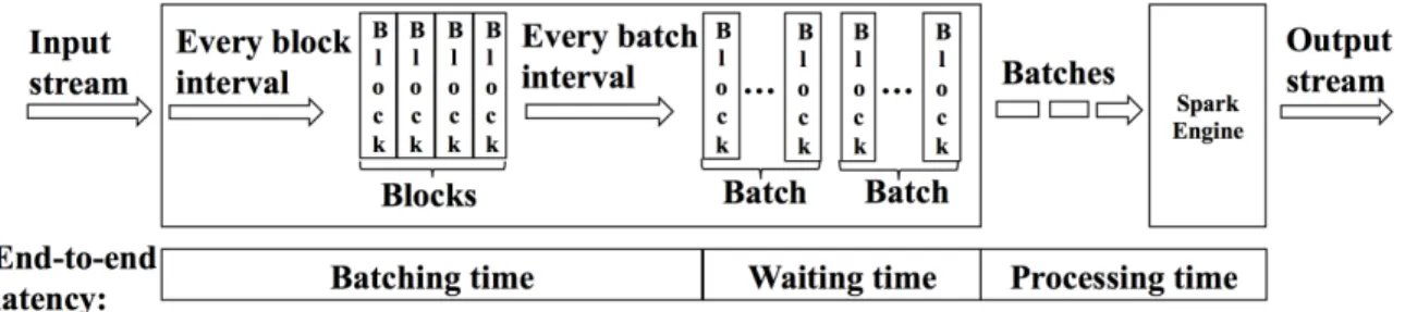
Figure 3.1: Stream processing model of Spark Streaming.
3.1
System Model
Spark Streaming is batched stream processing framework, which is a library extension on top of the large-scale data processing engine Apache Spark [51]. Figure 3.1 demon-strates a detail model of Spark Streaming. In general, Spark Streaming divides the con-tinuously input data stream into batches in discrete time intervals. To form a batch, two important parameters, block interval and batch interval are used to scatter the received data. First, the received data are split with a relatively small block interval (by default it is 200 milliseconds, and the minimal value it can take is 100 ms) to generate ablock. Then after very batch interval (by default it is 2 seconds, and minimal value it can take is 100 milliseconds), all the blocks in the block queue are dequeued and wrapped into a batch. Finally batches are put into a batch queue, and the spark engine will process them one by one. Basically, the batch interval determines the data size (i.e., number of data records), and the execution parallelism of a batch is defined as batch intervalblock interval, which is exactly the number of blocks in that batch. Based on such semantics, the end-to-end (E2E) latency consists of three parts:
• Batching time: The duration between the time a data record is received and the time that record is sent to batch queue;
relationship between batch interval and processing time;
• Processing time: The processing time of a batch, which depends on the batch interval and execution parallelism.
Note that the batching time is upper bounded by the batch interval. The waiting time could be infinitely large, and eventually some resources will be exhausted (e.g. OutOfMem-ory), which causes the system destabilized. Moreover, the process time is not only depends on the batch interval and execution parallelism but also the available resources of the pro-cess engine.
3.2
Requirements for Minimizing E2E Latency
Based on the definition of E2E latency, it is clear that the batch interval and execution parallelism have significant impact on the latency. However, both the batch interval and block interval are assigned only once before launching an application, and they keep static as long as the application instance lives. With such one-time setting only requirement, to make sure that the batched stream processing system can handle all workload under any op-erating situations (e.g., different cluster, unpredictable data surge), the desired interval need to be chosen either by offline profiling, or by sufficient resource provisioning. However, offline profiling is vulnerable to any change of available resource and workload, which requires multiple times of profiling whenever the operating condition changes. It is also hard to provision enough resources to handle unpredictable data surges, which is also not necessary for normal conditions that may dominate the most of running time. Furthermore, a statically set batch interval destabilize the system due to indefinitely increasing waiting time, which is obviously not the case to minimize latency. Therefore, the first requirement for minimizing latency is keeping the stability of the system, which essentially means on
To minimize the latency, a small batch interval is preferred since it means less data to process in the processing stage, which may also lead to less processing time. However, as aforementioned, the relationship between the batch interval and processing time depends on both workload characteristics and cluster configuration. The workload characteristics decide the upper bound of processing time in terms of time complexity and the cluster configuration determines how the computation is conducted. With the same batch interval, larger execution parallelism may incur less processing time and consequently reduce the total latency, but it is needless to be true always since larger parallelism also accompanies other overhead for task creation and communication. Thus, to minimize the latency, the second requirement is to identify how batch interval and execution parallelism affect the performance.
A fixed batch interval cannot guarantee the stability, and in the case of Spark Streaming, along with a fixed block interval, the execution parallelism is also static. Therefore, in this work, we propose to dynamically adjust the batch interval and block interval such that the system is stable as well as the latency is minimized. To keep the system stable, the sufficient condition is that the processing time of a batch must not exceed the batch interval on average. Note that it is not necessary to always keep the processing time less than batch interval for each batch to avoid building up of batch queue. To find such a batch interval that satisfies the stability condition and minimize the latency, we still need to identify the relationship between batch interval and processing time as well as the relationship between batch interval and processing time. Thus, we will discuss how the batch interval and block interval affect the latency in the following section.
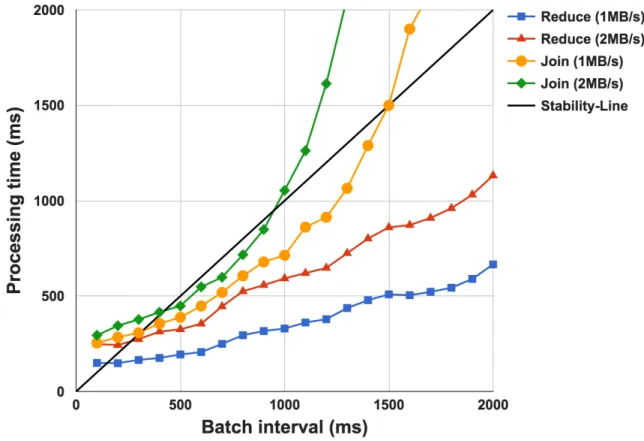
Figure 3.2: The relationships between processing times and batch interval of two streaming workloads with respect to batch intervals and data rates. The block interval is fixed to 100 ms.
3.3
Effect of Batch and Block Interval Sizing on Latency
In this section we first show the relationships between block interval and processing time for two representative streaming workloads. Then we further explore how block in-terval affects the processing time for the same workloads.
3.4
The Case for Batch Interval Sizing
Intuitively, the processing time should be a monotonically increasing function of batch interval, since the larger batch interval is, the more data should be processing. However,
nential), that depends on the characteristics of workload, input data rate, and the processing engine. Thus, we choose two representative streaming workload in the real world to ex-plore the relationship between batch interval and processing time. The first workload is
Reduce, which aggregates the received data based on keys. In the following of this thesis, we use networked word count as an example ofReduceworkload. The second one isJoin, which joins two different data streams.
Figure 3.2 illustrates the relationship between batch interval and processing time for
ReduceandJoinworkloads with different data injection rates, in which cases the block in-terval is set to 100 ms. Basically,Reduceshows a linear relationship between batch interval and processing time andJoinhas a super-linear behavior due to the potential computation complexity of O(M ×N) when two data streams are joined with M andN records re-spectively. For both workloads processing time varies with the input data rates, and with the same batch interval, larger data rates leads to higher processing time. The area below thestability-lineis the stable zone where the batch interval is larger than processing time. Note that with longer batch interval, Reduce has more stable operating status (i.e., batch interval is much larger than processing time), while the stable operating condition forJoin
is limited as larger batch interval leads to unstable operating zone. For both workload, the ideal batch interval is the smallest batch interval that meets the stability conditions, which can be identified by the point of intersection of thestability-line and thebatch interval -processing time lines. For linear workload (i.e., Reduce), there will be only one point of intersection, while for super linear workload (i.e., Join), multiple intersection points may exist. For super linear case, we expect our adaptive algorithm is able to find the lowest intersection point, which not only keeps the stability but also minimizes the latency.
3.5
The Case for Block Interval Sizing
As we discussed, the block interval indirectly determines the execution parallelism that significantly affect the performance on latency. In practice, the execution parallelism (e.g., number of tasks in a batch) is2−3times of the total number of processing cores [12, 13], such that all available resources are fully utilized. Intuitively, more parallelism may fully utilize the available resource and leads to less computation time. However, too much small tasks may also incurs more overhead of task creation, communication, and synchronization. Therefore, we explore that how block interval affect the processing time ofReduceandJoin
workloads.
Figure 3.3 illustrates the effect of block sizing on processing time for Reduce. Figure 3.3(a) shows the relationship between block interval and processing time for different batch intervals. We applied quadratic regression for each batch interval, and the optimal block interval is achieved around the extreme point of that parabola. For the same batch interval, the optimal block interval may be the same (i.e., 3200ms-6MB/s and 3200ms-4MB/s) or identical (2800ms-6MB/s and 2800ms-4MB/s) as shown in Figure 3.3(b). Note that we do not claim that the relationship between block interval and processing time is a quadratic function, and the only purpose we use quadratic regression is to show the trend. Undoubt-edly, the optimal block interval varies along with batch interval and data rate. Being aware of above observations, for a given batch interval that meets the stability condition, we can further reduce the E2E latency by using a block interval that minimize the processing time. To this point, we have explored how batch and block sizing affect the processing and consequently the E2E latency. In the next section, we introduce our online adaptive batch and block sizing algorithm that are designed according to these insights.
(a) The relationship between block interval and processing time when using different batch intervals with their corresponding trend lines (Quadratic). The data rate is 4 MB/s.
(b) The optimal block interval varies along with batch interval and data rate.
CHAPTER 4 DYBBS: DYNAMIC BLOCK AND BATCH
SIZING
In this section, we first address the problem statement that describes the goal of our control algorithm and remaining issues in existing solutions. Then we introduce how we achieve the goal and address the issues with isotonic regression and heuristic approach. Finally, we present the overall algorithm.
4.1
Problem Statement
The goal of our control algorithm is to minimize the end-to-end latency by batch and block sizing while ensuring the system stability. The algorithm should be able to quickly converge to the desired batch and block interval and continuously adapt batch and block interval based on time-varying data rate and other operating conditions. We also assume the algorithm has no prior knowledge of workload characteristics, which means the algorithm needs to learn with the information gathered from completed job statistics. Compared to the works in literature, we adapt both batch interval and block interval simultaneously, which is the most challenging part in the algorithm design. In addition to this major goal, we also wish to solve several issues existing in current solutions:
• Overestimation: Generally, a configurable ratio (e.g.ρ < 1) is used to relax the con-vergence requirements to cope with noise. In this case, a control algorithm converges
and processing time (i.e.,(1−ρ)×batch intervalincreases linearly along with the batch interval. This overestimation induce non-negligible increment on latency;
• Delay response: In ideal case, the waiting time is small and the control results re-spond to the operating conditions in near real-time manner. However, when the wait-ing time is large (e.g., few times of the batch interval), the statistics of the latest completed batch used to predict new batch interval is already out of date, which usually cannot reflect the immediate data ingestion rates. This long loop delay may temporarily further enlarge the waiting time and latency;
To achieve the major goal and address the issues, we introduce the batch sizing using isotonic regression and block sizing with heuristic approach, which are explained in detail in following two sections, respectively. Moreover, we concentrate the algorithm design for
ReduceandJoinworkloads. The case for other workloads is discussed in Section 7.
4.2
Batch Sizing with Isotonic Regression
For online control algorithms that model and modify a system at the same time suffer the trade-off between learning speed and control accuracy. The more information the al-gorithm learns, the higher accuracy can be achieved but longer convergence time is also required. We choose our algorithm to be accurate than fast convergence speed. The reason here is that compared to record-based stream processing system, batched stream system has relatively loose constraints in terms of convergence speed since the time duration be-tween two consecutive batches is at least the minimal batch interval that is available in that system. The control algorithm can learn and modify the system during that short duration. The minimal batch interval usually is at the magnitude of tens or hundreds milliseconds,
which means we have enough time to model the system with more complicated method. In the case of Spark Streaming, the minimal batch interval is 100 milliseconds, which is a long duration in terms of CPU time. Therefore, we choose to learn the system with a regression method.
Given that a time-consuming regression based algorithm can be used, an intuitive way to model the system is to directly use linear or superlinear function to fit a curve with statistics of completed batches. However, it requires prior knowledge of workload that violates our intention. As shown in Section 3 that the processing time is a monotonic increasing function of batch interval for both Reduce and Join, we choose a well-known regression techniques, Isotonic Regression [1], which is designed to fit a curve where the direction of the trend is strictly increasing. A benefit of isotonic regression is that it does not assume any form for the target function, such as linearity assumed by linear regression. This is also what we expect that using a single regression model to handle bothReduceand
Joinworkloads.
Using isotonic regression, our control algorithm is expected to model different work-loads without any assumption or prior knowledge of workload characteristics. Another benefit of using regression model is that the overestimation can be eliminated since we can find exact the lowest intersection point as long as the fitting curve is accurate enough. However, in reality noisy statistics may affect the accuracy of the fitting curve, and thus we still need to cope with noisy behavior. Compared to ratio based (e.g.,processing time < ρ×batch interval) constraint relaxing, we use a constant (e.g.,c) to relax the constraint, that is processing time + c < batch interval. With a constant difference between processing time and batch interval, the algorithm can converge as close as possible to the optimal point even with large batch interval value, in which case the ratio based method introduces a large overestimation.
and its corresponding processing time) of completed batches. Note that all the statistics data used for isotonic regression comes from batches that have the same block interval. Suppose the regression curve isIsoR(x), wherexis the batch interval, andIsoR(x)is the processing time. Then we identify the lowest point of intersection by finding the smallestx
such thatIsoR(x) +c < x. Since different data ingestion rates have identical relationship between processing time and batch interval, we then fit the curve for each identical data rate. Note that we do not need to examine all data ingestion rate to find the intersection point. We only fit the curve for the immediate data ingestion rate that is the same rate in the latest batch statistics as we assume the data ingestion rate keeps the same in the near future (within the next batch interval).
Till now we have explained the reason of choosing isotonic regression and how our algorithm addresses the overestimation issue. In the following section, we will introduce how our algorithm handles block sizing.
4.3
Block Sizing with Heuristic Approach
The block interval affects the E2E latency via its impact on execution parallelism. As we shown in Section 3, with a fix block interval, the best case a control algorithm can reach is actually a local optimal case in the entire solution space, which is far from the global optimal case that can significantly further reduce the E2E latency. Therefore, we wish our algorithm is able to explore all solution space through block sizing.
As aforementioned, the relation ship between block interval and processing time is not quadratic although we use it as the trend line in above results. Even though this relationship is quadratic, our control algorithm still need to enumerating all possible block intervals to find the global optimal case, which is the same as brute-force solution. Few reasons that we
cannot use quadratic regression are: i) In order to get all those initial sample statistics, the control algorithm have to try all possible block and batch intervals at the very beginning, which is not acceptable for an online control algorithm; ii) the time used for enumerating all possible block intervals may exceed the minimal block interval (e.g., 100 milliseconds in Spark Streaming), in which condition the real-time control requirement is not satisfied. Therefore, we propose a heuristic approach performing the block sizing to avoid enumera-tion and frequent regression computaenumera-tion.
Similar to the batch sizing, with different data ingestion rates, the curves of processing time and block interval are also identical. Thus, we use the same strategy used in batch sizing, which is that for each specific data rate we use the same heuristic approach to find the global optimal point. Basically, this heuristic approach start with the minimal block interval and gradually increase the block size until we cannot benefit from larger block interval. The detailed heuristic approach is described as following: i) Starting with the minimal batch interval, we use isotonic regression to find the local optimal point within that block interval (i.e., only applying batch sizing with a fix block interval); ii) Then increase the block interval by a configurable step size and apply the batch sizing method until it converges; and iii) If the E2E latency can be reduced with new block interval, then repeat step ii; otherwise the algorithm reaches the global optimal point. Besides, we also tracks all local optimal points for all block intervals that have been tried. Note that with the same data ingestion rate and operating condition, the global optimal point is stable. When the operation conditions change, the global optimal point may shift, in which case the algorithm needs to adapt to the new condition by repeating the above three steps. However, restarting from scratch slows down the convergence time, thus we choose to restart the above heuristic approach from the best suboptimal solution among all local optimal points to handle operating condition changing.
block sizing with a heuristic approach. The next step is to combine these two parts to form a practical control algorithm, which is discussed in next section.
4.4
Our Solution - DyBBS
Here we introduce our control algorithm - Dynamic Block and Batch Sizing(DyBBS) that integrates the discussed isotonic regression based batch sizing and heuristic approach for block sizing. DyBBS uses statistics of completed batches to predict the block interval and batch interval of the next batch to be received. Before we explain the algorithm, we first introduce two the most important data structures that are used to track the statistics and current status of the system. First, we use a table (denoted asStatsin the rest of this thesis) with entries in terms of a quadruple of(data rate, block intvl, batch intvl, proc time)to record the statistics, where thedata rateis the data ingestion rate of a batch,block intvlis the block interval of a batch,batch intvl is the batch interval of a batch, andproc timeis the processing time of a batch. Theproc timeis updated using weighted sliding average on all processing times of batches that have the samedata rate,block intvl, andbatch intvl. We also track the current block interval (denoted ascurr block intvl) last used for a spe-cific data ingestion rate by mappingdata rateto its correspondingcurrblock intvl, which
indicates the latest status of block sizing for that specific data rate, and this mapping func-tion is denoted asDR to BL.
Algorithm 1 presents the core function that calculates the next block and batch inter-val. The input of DyBBS is the data rate that is the data ingestion rate observed in the last batch. First, the algorithm gets the last used block interval of the data rate. Sec-ondly, all the entries with the same data rate and curr block intvl are extracted, which are used for functionIsoRto calculate the optimal batch interval, as shown on Line3and
Algorithm 1DyBBS-Dynamic Block and Batch Sizing Algorithm
Require: data rate: data ingestion rate of last batch
1: FunctionDyBBS(data rate)
2: curr block intvl = DR to BL(data rate)
3: (block intvl, proc time)[] = Stats.getAllEntries(data rate,curr block intvl)
4: new batch intvl = IsoR((block intvl, proc time)[])
5: proc time of new batch intvl = Stats.get(data rate, curr block intvl,
new batch intvl)
6: ifproc time of new batch intvl +c <new batch intvlthen
7: if curr block intvl is the same of block interval of current global optimal point
then
8: new block intvl = curr block intvl + block step size
9: else
10: new block intvl is set to the block interval of the best suboptimal point
11: endif
12: else
13: new block intvl = curr block intvl
14: endif
15: Update(new block intvl,new batch intvl)
16: EndFunction
4. Thirdly, the algorithm compares the estimatednew batch intvland the sliding averaged
proc time. We treat the isotonic regression result converges if the condition on Line 6is true and then the algorithm will try different block interval based on operating condition. If thecurr block intvlis as the same as that of the global optimal point stated on Line7, then increase the block interval by certain step size. Otherwise, we treat it as the operating condition changing and choose the block interval of the suboptimal point. If the condition on Line 6is not satisfied (Line12), it means theIsoR forcurr block intvl has not con-verged and then keep the block interval unchanged. Finally, DyBBS updates the new block interval and batch interval. Note that thenew batch intvlis always rounded to a multiplier of thenew block intvl, which is omitted in the above pseudo code. In addition, when the
IsoR is called, if there is less than five samples points (i.e., the number of unique batch intervals is less than five), it will return a new batch interval using slow-start algorithm [44]. With almost full history statistics (except the batches still in the queue), DyBBS can avoid
related statistics in history instead of recently completed batches statistics.
In this section, we have introduced our adaptive block and batch sizing control algo-rithm and showed that our algoalgo-rithm can handle the overestimation and long delay issues. We will discuss the implementation of DyBBS on Spark Streaming.
CHAPTER 5 IMPLEMENTATION
We implement our dynamic block and batch sizing algorithm in Spark Streaming (ver-sion 1.4.0), which is a open-source distributed batched stream processing system. Basi-cally we change the behavior of batch generation. Instead of generating batch with the same batch size, DyBBS generates batches with different sizes. Figure 5.1 illustrates the high-level architecture of the customized Spark Streaming system. We modified theBlock Generator and Batch Generator modules such that they can generates different size of blocks and batches based on the control results. We first introduce the statistic gathering module to get the statistics of completed batches. Then, we add the DyBBS module to pre-dicts the next batch size and execution parallelism. The new execution parallelism is used byBlock Generatormodule to determine the number of tasks of the new batch. The batch size is used to generate a batch with the new size byBatch Generatormodule. In theBatch Processor module, we added the functionality of gathering statistics of each completed batch. We also introduced a new module ofDyBBSthat implements our control algorithm utilizing the batches statistics. The detailed modifications are as follows:
• Block Generator: This module generates relatively small blocks based on the block interval. To apply the new execution parallelism, we need to change the block interval such that the number of blocks could be the one that minimizes the latency with the new batch interval. We modified the behavior of the timer used to continuously generates blocks. Since the timer ofBlock Generatoris on the data receiver, so when
Figure 5.1: High-level overview of our system that employs DyBBS.
we change the time duration of timer interruption, the driver program has to send the new block interval to all receivers. This involves additional communication between driver program and data receivers. This is implemented by adding a new actor based message to existing communication module. The generated blocks are handled off to the batch generator.
• Batch Generator: This module generates batches using blocks. Similar toBlock Gen-erator, we also changed the timer behavior such that it can generate a batch with new batch interval. Whenever the batch generator’s times is changed, the driver program also sends the new block interval via message passing as described above. The timer behavior changing is conducted in theschedulermodule of Spark Streaming, which generates batches and submits the job toBatch Processor.
• Batch Processor: The module is unmodified, and the statistics are sent to DyBBS. The statistics are available in the native Spark Streaming, and we just gather the ones DyBBS needs.
• DyBBS: In this module we implemented our adaptive block and batch sizing algo-rithm that takes the batches statistics as input and calculates the new block interval and batch interval.
Table 5.1: The modules and files that have been modified.
Module File path
dstream $SPARK HOME\streaming\src\main\scala\org\apache\spark\streaming
\dstream\DStream.scala
receiver $SPARK HOME\streaming\src\main\scala\org\apache\spark\streaming
\receiver\ReceiverSupervisorImpl.scala
$SPARK HOME\streaming\src\main\scala\org\apache\spark\streaming
\receiver\ReceiverMessage.scala
$SPARK HOME\streaming\src\main\scala\org\apache\spark\streaming
\receiver\BlockGenerator.scala
$SPARK HOME\streaming\src\main\scala\org\apache\spark\streaming
\receiver\Receiver.scala
scheduler $SPARK HOME\streaming\src\main\scala\org\apache\spark\streaming
\scheduler\IsoRegression.scala
$SPARK HOME\streaming\src\main\scala\org\apache\spark\streaming
\scheduler\JobGenerator.scala
$SPARK HOME\streaming\src\main\scala\org\apache\spark\streaming
\scheduler\ReceiverTracker.scala
$SPARK HOME\streaming\src\main\scala\org\apache\spark\streaming
\scheduler\JobSet.scala
others $SPARK HOME\streaming\src\main\scala\org\apache\spark\streaming
ing source code. In total, we modifies about 300 lines of code of original codes to support our dynamic block and batch sizing. We also introduced roughly 500 lines of code to implement DyBBS in Spark Streaming.
There are three configurable parameters used in our algorithm. The first one is constant
c used to relax the stability condition. Largerc keeps the system more stable and more robust to noisy, but also leads to larger latency. The second parameter is block interval incremental step size. Larger step size incurs fast convergence speed on block sizing pro-cedure. However, it may also never converge to the global optimal case due to too large step size. The last parameter is used for data ingestion rate discretization. In DyBBS, the isotonic regression are conducted on batch interval and processing time for s specific data rate. In our algorithm, we first get the data rate of each batch in terms of megabytes per second. Then we discretize the data rate by a configurable step size. This discretization granularity could be different under different operating condition. All those three param-eters can affect the performance of our control algorithm, and in our implementation, we choose50ms the constant valuec, 100ms for the block step size, and0.2MB/s for the data rate discretization.
In summary, our modifications do not require any changes to the user’s program or programming interfaces. Although our implementation is Spark Streaming specified, it is easy to implement our control algorithm on other batched stream processing systems that have similar design principle of block and batch.
CHAPTER 6 EVALUATION
We evaluate the DyBBS withReduceandJoinstreaming workloads under various com-binations of data rates and operating conditions. Our results show that DyBBS is able to achieve latencies comparable to the optimal case. The comparison with the other two prac-tical approaches illustrates that our algorithm achieves the lowest latency. We demonstrates that the convergence speed our algorithm is slower than the state-of-art only for the first time a data rate appears, and for the second and following appearance of the same data rate our algorithm is much faster. Finally we also show our algorithm can adapt to resource variation.
6.1
Experiment Setup
In the evaluation, we used a small cluster with four physical nodes. Each node can hold four Spark executor instances (1 core with 2 GB memory) at most. We ran two workloads as mentioned-Reduceand Join, with two different time-vary data rate patterns. The first data rate pattern is sinusoidal fashion of which the data rate varies between 1.5 MB/s to 6.5 MB/s forReduce, and 1 MB/s to 4 MB/s forJoin, with periodicity of 60 seconds. The other one is Markov chain [2] fashion of which the data rate changes every 15 seconds within the same rate duration as sinusoidal fashion. For the input data, we generated eight bytes long random strings as the key for reducing and join operations, and the number of uniques key is around32,000. The output is written out to a HDFS file [43].
(a) Comparison for Reduce with sinusoidal in-put.
(b) Comparison forJoinwith sinusoidal input.
(c) Comparison for Reduce with Markov chain input.
(d) Comparison forJoinwith Markov chain In-put.
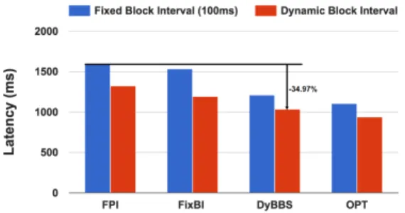
Figure 6.1: The performance comparison of average E2E latency over 10 minutes for Re-duce andJoin with sinusoidal and Markov chain input rates, for four approaches of FPI, FixBI, DyBBS, and OPT.
As comparison, we implemented three other solutions that are as follow:
• FPI: This is the only one of practical solution so far that adopts fix-point iteration (FPI) to dynamically adapt batch interval in Spark Streaming [14].
• FixBI: We compare our algorithm with this unpractical hand-tuning method. It takes the best case (i.e., with the lowest average latency over entire running duration) by enumerates all possible pair of block and batch intervals. However, it still uses static setting over the running time and cannot change either block or batch interval at runtime.
• OPT: This is the oracle case, that we dynamically change the block and batch interval at the runtime based on prior knowledge.
For the performance experiments, we implemented two different versions for each of above three methods: i) the batch-only version changes the batch interval while keeps the block interval fixed (i.e., 100ms); and ii) the second version adapts both block and batch intervals, which is also the object our algorithm designed for. For FPI that is not designed for block sizing, we set a block interval based on prior knowledge such that it achieves local optimal with the batch interval FPI suggests. To support the batch-only algorithm in DyBBS, we set the block interval to 100ms and disable the block sizing only for the second version algorithm. The E2E latency of a batch is defined as the summation of batch interval, waiting time, and processing time. In all following experiments, we used the average value of all E2E latencies over entire experiment as the criteria for performance comparison.
6.2
Performance on Minimizing Average E2E Latency
We compared the average E2E latency over 10 minutes forReduceandJoinworkloads with sinusoidal and Markov chain input rates. In each case, we run two different control algorithms that are denoted asFixed Block Interval (100ms)andDynamic Block Interval. Figure 6.1 shows that our DyBBS achieves the lowest latencies that is comparable with the oracle case (OPT). In general, by introducing block sizing, the latency is significantly reduced compared to that only applies batch sizing. As Figure 6.1 showed, our DyBBS outperforms the FPI and FixBI in all cases. Specifically, compared with FPI with fixed block interval, our DyBBS with dynamic block interval reduced the latencies by 34.97% and 48.02% forReduceworkload with sinusoidal and Markov chain input rates (the cases in Figure 6.1(a) and 6.1(c)), respectively. For Join workload, our DyBBS with dynamic block interval reduced the latencies by 63.28% and 67.51% for sinusoidal and Markov chain input rates respectively (the cases in Figure 6.1(b) and 6.1(d)), compared to FPI with
two folds: i) In terms of batch interval sizing, DyBBS achieves lower overestimation due to the more accurate regression model; and ii) In terms of block tuning, DyBBS dynamically change the block size based on the workload variation rather than either block interval resizing correlated to the batch interval used in FPI or hand-tuning enumeration used in FixBI.
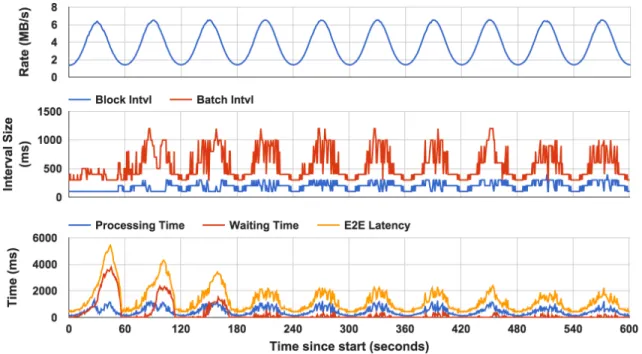
In terms of real-time performance, Figure 6.2 shows the dynamic behaviors including block interval, batch interval, waiting time, processing time, and E2E latency forReduce
workload with sinusoidal input, for DyBBS. During the first three minutes (the first three sine waves), our algorithm was learning the workload characteristics, and hence the latency is relatively high. After our algorithm converged (from the fourth minute), the latency is relatively low and maintained the same for the rest of time. Especially, in the first minute, the block interval is always the same and the batch interval is relatively small since that the block interval is initialed with 100ms and the batch interval uses slow start algorithm. From the second minute, our algorithm activates the block sizing procedure, and eventually the block interval and batch interval converges after certain learning time. In Figure 6.3, we compared the batch interval and E2E latency of FPI and DyBBS. During the first 60 seconds, the E2E latency of DyBBS is higher than FPI due to imprecise isotonic regression model. In the next two periodicities, the E2E latency of DyBBS reduces since the isotonic regression model is becoming more and more accurate.
6.3
Convergence Speed
In our design, we chosen to make the control algorithm accurate in the trade-off between accuracy and fast convergence speed. We first compared the convergence speed ofReduce
Figure 6.2: The DyBBS’s real-time behavior of block interval, batch interval, waiting time, processing time, and E2E latency forReduceworkload with sinusoidal input data rate. block sizing, we only present the behavior of batch interval along with the data rate in Figure 6.4. The data rate starts with 1MB/s and jumps to 3MB/s after 5 seconds (the first black dashed vertical line from the left), then it steps down to 1MB/s at 30th seconds (the second black dashed vertical line from the left) and back to 3MB/s again after 45 seconds (the third black dashed vertical line from the left). Before the star time, we run FPI and DyBBS long enough such that both of them have converged with the 1MB/s data rate. Thus, for the first five seconds, the block interval are constant. At the 5th second, the data rate changes to 3MB/s, that is the first time the rate appears during entire experiment. Then FPI and DyBBS start to adapt the batch interval. The FPI first converges after roughly at 11th seconds (the red vertical line on the left), while DyBBS converges until 18th seconds (the blue vertical line on the left). This is caused by the longer learning time of isotonic regression used in DyBBS. When both FPI and DyBBS converged, DyBBS has smaller convergence value than FPI due to more accurate regression model used by DyBBS. When
Figure 6.3: Comparison of batch interval and E2E latency of FPI and DyBBS forReduce
workload with sinusoidal input data rate.
the second time that the data rate changes to 3MB/s, in contrary to the first time, our DyBBS converges first at 47th second (the blue vertical line on the right), while FPI converges seven seconds later (the red vertical line on the right). Since FPI only uses the statistics of last two batches that means it cannot leverage historical statistics, hence FPI has to re-converge every time the data rate changes. However, our DyBBS has all the historical statistics (in Statstable) and quickly locate the convergence value. Thus, for a specific data rate, DyBBS has long convergence time for the first time that rate appears and extremely small convergence time for the second and rest times the same data rate appears.
With block sizing enabled in DyBBS, the convergence time is longer than that when block sizing is disabled. Figure 6.5 shows the convergence time forReduceworkload with two different constant data rates. With larger data ingestion rate, our algorithm spent more time to search for the optimal point since there are more potential candidates. Specifically, when the data rate is 3MB/s as shown in Figure 6.5(a), the convergence time is less than 20 seconds, and our algorithm only explored three different block intervals (100ms, 200ms,
Figure 6.4: Timeline of data ingestion rate and batch interval for Reduceworkload using FPI and DyBBS with fixed block interval. Our algorithm spent longer time to converge for the first time a specific rate occurs, but less time for the second and later times that rate appears.
and 300ms). When the data rate is 6MB/s as shown in Figure 6.5(b), DyBBS spent more than 30 seconds to explore the block interval from 100ms to 400ms. Although our algo-rithm spends tens of seconds to converge for large data ingestion rate, this convergence time is relatively small compared to the execution time (hours, days, even months) of long run streaming application. Therefore, we believe that our algorithm is able to handle large data ingestion rate for long run applications.
6.4
Adaptation on Resource Variation
In above experiments, we have showed that our algorithm is able to adapt to vari-ous workload and workload variation. We also argued that when the operating condition changes, our algorithm should detect the resource variation and adjust the block and batch interval consequently. It is common that the available resources for stream processing job
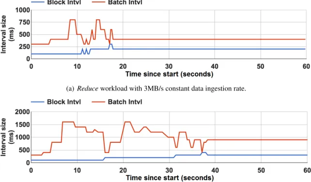
(a) Reduceworkload with 3MB/s constant data ingestion rate.
(b) Reduceworkload with 6MB/s constant data ingestion rate.
Figure 6.5: Timeline of block interval, batch interval for Reduceworkload with different data ingestion rates using DyBBS with block sizing. Larger data ingestion rate leads to longer convergence time.
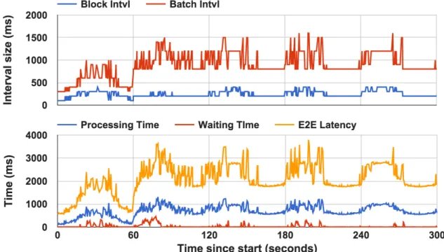
is reduced due to job submissions by other applications on a shared cluster. To emulate the resource reduction, we run a background job on one of the four nodes such that the node is fully occupied by the background job, which equivalently reduces the available resource via removing that node. Figure 6.6 illustrates that our algorithm can adapt the resource reduction (at 60th second) by increasing the batch interval and E2E latency. Our algorithm took another tree minutes to adapt to the new operating condition. Note that, our algorithm did not restart from the scratch by retrying the block interval from 100ms.
Figure 6.6: Timeline of block interval, batch interval, and other times forReduceworkload under resource variation. At the 60th second, external job takes away 25% resources of the cluster.
CHAPTER 7 DISCUSSION
In this thesis, we narrowed down the scope of our algorithm to two workloads with sim-ple relationships (i.e., linear forReduceand superlinear forJoin). There may be workload with more complex characteristics thanReduceandJoin. An example of such workload is
Windowoperation, which aggregates the partial results of all bathes within a sliding win-dow time duration. This issues is also addressed in [14], and the Window operations is handled by using small mini-batch with 100ms interval. In our approach, there are two problems for handlingWindowworkload. One problem is that it is possible that we cannot find a serial of consecutive batches such that the total time interval exactly equals the win-dow duration. If we always choose the next batch interval such that the previous condition is satisfied, then we lose the opportunity to optimize that batch, as well as all the batches in the future. Another problem is that our approach dynamically changes the block size, which means our approach cannot directly employs the method used in [14] that treats a block as a mini-batch. Therefore, we leave the work to supportWindowworkload for the future.
CHAPTER 8 CONCLUSION
In this thesis, we have illustrated an adaptive control algorithm for batched processing system by leveraging dynamic block and batch interval sizing. Our algorithm is able to achieve latencies without any workload specific prior knowledge, which are comparable to the oracle case due to our accurate batch interval estimation and novel execution parallelism tuning. We have shown that our algorithm can reduce the latencies by at least 34.97% and 63.28% for Reduce and Join workloads respectively, and have presented the abilities of DyBBS to adapt to various workloads and operating conditions.