L-classifier chains classification and variable selection for multi-label datasets

(1)

Monika du Toit

Thesis presented in partial fulfillment of the requirements for the degree of MCom (Mathematical Statistics) at the University of Stellenbosch

December 2016

(2)

ii

Plagiarism declaration

1. Plagiarism is the use of ideas, material and other intellectual property of another’s work and to present it as my own.

2. I agree that plagiarism is a punishable offence because it constitutes theft. 3. I also understand that direct translations are plagiarism.

4. Accordingly all quotations and contributions from any source whatsoever (including the internet) have been cited fully. I understand that the reproduction of text without quotation marks (even when the source is cited) is plagiarism. 5. I declare that the work contained in this assignment, except otherwise stated, is

my original work and that I have not previously (in its entirety or in part) submitted it for grading in this module/assignment or another module/assignment.

Signature

Initials and surname M du Toit Date December 2016

(3)

iii

Abstract

Multi-label classification extends binary and multi-class classification to scenarios where every data case is assigned several labels simultaneously. Applications include labelling images with tags, identifying instruments that are playing in a musical piece and classifying text according to two or more labels. Variable selection is an important part of multi-label data analysis, but it has received little attention in the literature. Multi-label variable selection is more complex than for binary classification, mainly due to the presence of more than one response as well as label dependence.

In this thesis, a multi-label classification approach called L-classifier chains (LCC) is proposed. This method implements a compromise between simple classifier chains and the ensemble of classifier chains procedures. The LCC approach uses an ensemble of classifier chains with a semi-random chain structure and random forests as base learners to perform variable selection. The specific structural assumptions of the LCC method allow for variable importance inference based on the output from the random forests. The results from LCC include multi-label predictions and a matrix of variable importance values.

This thesis illustrates the application of the LCC clasifier by conducting empirical work using multi-label benchmark datasets, simulated datasets and a practical dataset obtained from a South African credit bureau. Throughout the practical applications, it compares the performance of LCC relative to three other classifiers, namely binary relevance, classifier chains and ensemble of classifier chains.

Key words:

(4)

iv

5.1 Introduction ... 57 5.2 Datasets ... 57 5.3 Experimental design ... 58 5.4 Exploratory analysis ... 59 5.4.1 Emotions dataset ... 59 5.4.2 Scene dataset ... 65 5.4.3 Yeast dataset ... 69 5.5 Confirmatory analysis ... 74 5.5.1 Friedman’s test ... 74 5.5.2 Post-hoc tests ... 75 5.6 Conclusion ... 77

CHAPTER 6: Multi-label simulation analysis ... 79

6.2 Simulation analysis ... 79

6.3 Datasets ... 80

(6)

vi

6.5 Exploratory analysis ... 85

6.5.1 Boxplots ... 85

6.5.2 L-classifier chains: heatmaps ... 95

6.5.3 L-classifier chains: identifying relevant variables ... 103

6.6 Confirmatory analysis ... 106

6.7 Conclusion ... 110

CHAPTER 7: Credit bureau dataset analysis ... 112

7.2 Dataset ... 112

7.3 Experimental design ... 115

7.4 Results ... 119

7.5 Variable importance results ... 125

7.6 Conclusion ... 132

CHAPTER 8: Conclusion and future research ideas ... 134

REFERENCES ... 137

APPENDIX A: Chapter 3 ... 141

A.1 Importance of the label sequence order ... 141

A.2 Comparison of classification methods ... 142

APPENDIX B: Chapter 5 ... 148

B.1 Benchmark analysis: classification ... 148

B.2 Benchmark analysis: exploratory analysis ... 153

APPENDIX C: Chapter 6 ... 156

C.1 Simulation analysis: classification ... 156

C.2 Simulation analysis: exploratory analysis ... 158

APPENDIX D: Chapter 7 ... 161

D.1 Data preparation and splitting ... 161

D.2 Screening of predictors ... 163

D.3 Comparison of classifiers ... 165

(7)

vii

List of figures

Figure 2.1 Summary of multi-label classification methods. Figure 3.1

Figure 3.2

Illustration of the CC training algorithm with four chain links.

CC classification of the emotions dataset using all label permutations.

Figure 3.3 Summary of classifier chains modifications. Figure 4.1 Classifier tree structure.

Figure 5.1 Emotions dataset: boxplots of ML evaluation measures for the four classifiers.

Figure 5.2 Emotions dataset: distribution of importance values for the LCC classifier.

Figure 5.3 Emotions dataset: heatmap of importance values for LCC classifier. Figure 5.4 Scene dataset: boxplots of ML evaluation measures for the four

classifiers.

Figure 5.5 Scene dataset: distribution of importance values for the LCC classifier.

Figure 5.6 Scene dataset: heatmap of importance values for the LCC classifier. Figure 5.7 Yeast dataset: boxplots of ML evaluation measures for the four

classifiers.

Figure 5.8a Yeast dataset: distribution of importance values for the LCC classifier.

Figure 5.8b Yeast dataset: distribution of importance values for the LCC classifier.

Figure 5.9 Yeast dataset: heatmap of importance values for the LCC classifier. Figure 6.1 Distribution of ML evaluation measures for all simulation designs

using the LCC classifier.

Figure 6.2 Distribution of ML evaluation measures for ρ: 0.1 vs 0.8 (Simulation 25 vs 27).

Figure 6.3 Distribution of ML evaluation measures for N_"#$%&: 200 vs 1000 (Simulation 1 vs 17).

Figure 6.4 Distribution of ML evaluation measures for P: 50 vs 100 (Simulation 23 vs 31).

(8)

viii Figure 6.5 Distribution of ML evaluation measures for L: 5 vs 20 (Simulation

19 vs 23).

Figure 6.6 Distribution of ML evaluation measures for t: 0.5 vs 5 (Simulation 13 vs 14).

Figure 6.7 Heatmap plots of variable importance values for ρ: 0.1 vs 0.8 (Simulation 29 vs 31).

Figure 6.8 Heatmap plots of variable importance values for N_"#$%&: 200 vs 1000 (Simulation 11 vs 27).

Figure 6.9 Heatmap plots of variable importance values for P: 50 vs 100 (Simulation 8 vs 16).

Figure 6.10 Heatmap plots of variable importance values for L: 5 vs 20 (Simulation 27 vs 31).

Figure 6.11 Heatmap plots of variable importance values for t: 0.5 vs 5 (Simulation 19 vs 20).

Figure 7.1 Distribution of the number of accounts per client. Figure 7.2 Densities of accounts in the credit bureau dataset. Figure 7.3 Distribution of the R)_values.

Figure 7.4 Evaluation measures for different threshold values. Figure 7.5 ROC curves for labels 2 and 3 for the credit bureau data. Figure 7.6 Heatmaps for the credit bureau data.

Figure 7.7 Variable importance plot for the credit bureau data.

(9)

ix

List of tables

Table 2.1 Summary of classification types. Table 2.2 Multi-label dataset structure.

Table 2.3 Illustration of six ML evaluation measures for three scenarios. Table 2.4 Binary relevance method.

Table 2.5 Label powerset method. Table 2.6 Pairwise method.

Table 3.1 ML classification of the emotions dataset using the BR, CC and 1-CC algorithms.

Table 3.2 Limitations of CC-based methods. Table 3.3 Training phase of the LCC method.

Table 3.4 Matrixof variable importance values for the CC classifier, 𝑨. Table 3.5 Matrix of variable importance values for the LCC classifier, 𝑨_,%&$-. Table 5.1 Summary of benchmark datasets used in experimental study. Table 5.2 Friedman’s test for benchmark datasets analysis.

Table 5.3 Bonferroni-Dunn’s test for the benchmark datasets analysis. Table 5.4 Holm’s post-hoc test for benchmark datasets analysis. Table 6.1 ML dataset generation: controlling parameters. Table 6.2 Structure of the simulation design.

Table 6.3 The proportion of correctly identified relevant variables by the LCC, VI_0#10.

Table 6.4 Friedman’s tests for the simulations analysis.

Table 6.5 Summary of the mean ranks of Friedman’s tests based on all evaluation measures.

Table 7.1 Summary of the credit bureau dataset.

Table 7.2 Distribution of number of accounts per client. Table 7.3 Summary of the R)_{distribution.}

Table 7.4 Threshold specification and corresponding number of predictors. Table 7.5 Credit bureau classification results for 15 labels.

Table 7.6 Confusion matrix.

(10)

x Table 7.8 The 10% globally most important predictors and their Gini index

values.

Table 7.9 Summary of the five most important predictors and the corresponding index values for each label.

(11)

xi

List of appendices

APPENDIX A Chapter 3

A.1 Importance of the label sequence order A.2 Comparison of classification methods

APPENDIX B Chapter 5

B.1 Benchmark analysis: classification

B.2 Benchmark analysis: exploratory analysis

APPENDIX C Chapter 6

C.1 Simulation analysis: classification C.2 Simulation analysis: exploratory analysis

APPENDIX D Chapter 7

D.1 Data preparation and splitting

D.2 Screening of predictors

D.3 Comparison of classifiers

(12)

xii

List of abbreviations and/or acronyms

AA Algorithm adaptation

AC Accuracy

BR Binary relevance

CC Classifier chains CL Classification accuracy ECC Ensemble classifier chains

F2 F2 score

HL Hamming loss

LCC L-classifier chains

LP Label powerset

ML Multi-label

PPT Pruned problem transformation

PR Precision

PT Problem transformation

RE Recall

RF Random forests

(13)

1

CHAPTER 1: Introduction

1.1 BACKGROUND

Supervised statistical learning refers to a set of approaches for estimating a functional relationship 𝑓 𝒙 between a set of input variables X and an output Y, in order to find a prediction rule for new input values 𝒙₄:

𝑓: 𝑿 → 𝑌 𝑿 , 𝑦 = 𝑓(𝒙₄).

For quantitative response variables, regression analysis techniques are applied. Alternatively, qualitative responses require the use of classification analysis. In regression, the functional relationship 𝑓 𝒙 = 𝐸(𝑌|𝑿 = 𝒙) is the expected value of the conditional distribution. Since the value of 𝑓 𝒙 is typically unknown,

𝐸 𝑌 𝑿 = 𝒙 needs to be estimated. In classification with two classes, it is of interest

to compute the predictions 𝐺 𝒙 = 𝑎𝑟𝑔𝑚𝑎𝑥_F𝑓 𝑔|𝒙 , 𝑔 ∈ 0,1 . The functional relationship in this case determines the threshold value for prediction rules. Depending on the model, it may refer to the estimated Bayes posterior probability or the majority class in a given cluster, for example. Classification will be the main focus of this thesis.

There exists a trade-off between the prediction accuracy and interpretability of a model. In classification, less flexible approaches such as logistic regression are restricted in terms of estimating 𝑓 𝒙 . These methods tend to have lower variance but potentially higher bias than more complex models. Interpretability of such models is often good. More flexible approaches, such as classification trees, model a wider variety of shapes of 𝑓 𝒙 . They often have lower bias, potentially higher variance and can provide limited inference. Deciding on the form of 𝑓 𝒙 becomes more difficult as the dimensionality and complexity of datasets increase.

The objective of this thesis is to consider a specific type of classification, multi-label (ML) classification, where each observation is associated simultaneously with more than one binary label. The thesis will focus on introducing an ML classification

(14)

2 method, as well as exploring variable selection (VS) and variable importance within this context.

1.2 NOTATION

The general notation in the ML context is focused on two sets of variables. Consider an ML training dataset of size N, consisting of P predictors and L binary labels. Let a set of responses or labels in this dataset be denoted by 𝒀 = 𝑌_L, 𝑌₎, … , 𝑌_N . Similarly, a set of input features, which refer to the variables conveying information about the labels, is 𝑿 = 𝑋_L, 𝑋₎, … , 𝑋_P . A training ML dataset is denoted by 𝒙_Q, 𝒚_{Q QSL}T _, where 𝒙_Q: 1×𝑃 is a feature vector of P predictors and 𝒚_Q: 1×𝐿 is a response vector of L binary labels, corresponding to observation i. The matrix representation of the ML dataset is 𝑿: 𝑁×𝑃 and 𝒀: 𝑁×𝐿. The columns of an observed data matrix 𝑿 and 𝒀 are denoted by N-dimensional vectors 𝒙_L, 𝒙₎, … , 𝒙_Pand𝒚_L, 𝒚₎, … , 𝒚_N respectively.

1.3 OVERVIEW

This thesis is divided into eight chapters, out of which the first and the last chapters consist of the introductory and conclusion chapters. The body of the thesis is split into theoretical Chapters 2, 3 and 4, and Chapters 5, 6 and 7, which describe the empirical work done.

Chapter 2 describes ML classification in general, starting with the distinction between the main classification types. It zooms in on ML classification and provides a description of some of the key characteristics of this problem. Furthermore, the objective of this thesis is also provided in this chapter. Finally, some of the most significant ML classification approaches are summarised and described.

The focus of Chapter 3 is on one of the ML classification methods known as classifier chains. Various aspects of this classifier are discussed, including its modifications and limitations, supported with some experimental work. In this chapter, the LCC algorithm is proposed and its most important aspects are explained in detail. Lastly, the implementation of VS within the LCC classifier is described.

(15)

3 Variable selection is the primary focus of Chapter 4. In this chapter, some of the problems associated with high-dimensional problems are discussed, followed by ways of overcoming them. A brief overview of existing VS methods is provided, followed by a summary of VS methods in ML classification. Special attention is paid to embedded VS methods, namely decision trees, bagging and random forests (RF). Furthermore, the concept of variable importance is explored within the RF model. Lastly, RF application in the proposed LCC classifier is described.

In Chapter 5, the benchmark datasets analysis is presented. It is the first part of the experimental work done in this thesis. In this analysis, three ML benchmark datasets are analysed using four ML classifiers, including the LCC classifier. The main idea of using these datasets is to apply some of the ML techniques to datasets available online. The objective of this analysis is to compare the accuracy of predictions of these classifiers. The comparison is done using various exploratory and confirmatory analyses of the results. Furthermore, the variable importance values from the LCC classifier are analysed.

The second part of the experimental work is summarised in Chapter 6. In this chapter, a simulation study was done in order to compare the ML classifiers in a controlled environment. This study consists of 32 simulation designs, each of which has varying values of the five parameters of interest. Exploratory, as well as confirmatory analyses of the ML classification results are provided. Lastly, the variable importance values from the LCC classifier’s output are explored within the different simulation designs.

In Chapter 7, the final part of the experimental work is presented. In this chapter a practical ML classification dataset obtained from a South African credit bureau is analysed. Of interest is to compare the performance of the four classifiers in an applied setting. Lastly, the importances of the predictors are analysed using variable importance values obtained from the LCC classifier.

(16)

4

CHAPTER 2: Multi-label classification

Classification in the context of multi-label data problems has stirred up interest in the last decade. Compared to simple binary classification, it offers larger scope for analysis due to the complexity of ML datasets. The concept of conditional label dependence is one of the main factors underlying the dataset structure. Applications of ML classification include the areas of image and text annotation, bioacoustics and bioinformatics.

2.1 CLASSIFICATION HIERARCHY

Classification is a statistical method supervised by a qualitative output. Its categories include binary, multi-class, multi-label and multi-output classification. The main distinction between these categories is in the format of the output.

As the name suggests, binary classification is associated with a single two-class response variable. A binary dataset is of the form:

(𝒙_Q, 𝑦_Q)_QSLT _, _𝒙

Q ∈ ℝP, 𝑦Q ∈ 0, 1 .

Extensive research has been done in this context. Generally, a method tries to identify a classification rule and determine which of the two classes is more likely to be associated with a given input. This decision rule can be linear (for example, linear discriminant analysis), non-linear (for example, RF) or linear in an extended feature space (for example, support vector machines). Many of these classifiers estimate the posterior probabilities and classify observations to the class with the highest estimated posterior probability:

𝑃 𝑌_Z 𝒙 =𝑓 𝒙, 𝑌Z

𝑓 𝒙 , 𝑗 ∈ 0, 1 , 𝑌 = 𝑎𝑟𝑔𝑚𝑎𝑥Z∈ 4,L 𝑃 𝑌Z 𝒙 .

Fraud detection, medical testing and quality control are examples of binary classification.

(17)

5 In multi-class classification every data case belongs to one of 𝐾 mutually exclusive classes. Examples of multi-class datasets include vowel recognition and multiple-type cancer classification. A multi-class dataset can be represented in the following way:

(𝒙_Q, 𝑦_Q)_QSLT _, _𝒙

Q ∈ℝP, 𝑦Q ∈ 1,2, … , 𝐾 , 𝐾 ≥ 3.

Multi-label classification can be identified by a set of L binary class labels that are non-mutually exclusive. Therefore, each observation can be associated with more than one label. Some of the well known applications include image annotation, text categorisation and music instrument recognition. An ML dataset has the following notation:

(𝒙_Q, 𝒚_Q)_QSLT _, _𝒙

Q ∈ℝP, 𝒚Q ∈ 0, 1 N , 𝐿 ≥ 2.

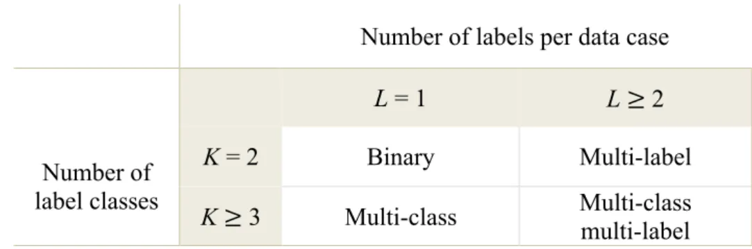
Lastly, a combination of L labels each consisting of K label classes is referred to as multi-class multi-label or multi-output classification. It is the most complex type of classification dataset. Examples of such a problem include Wikipedia page label tags and Flickr photo label tags (Dekel, 2010). The classification hierarchy is summarized in Table 2.1.

Table 2.1: Summary of classification types

Number of labels per data case L = 1 L ≥ 2 Number of

label classes

K = 2 Binary Multi-label K ≥ 3 Multi-class Multi-class _multi-label

(18)

6

2.2 COMPLEXITY OF MULTI-LABEL DATASETS

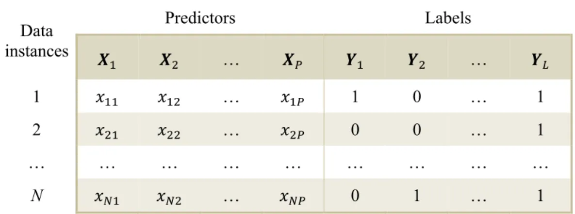
In the last decade research on ML classification has experienced significant growth. However, compared to well-researched binary classification, ML classification is still more of an unchartered type of problem. Some approaches are better known than others, but in general a standard procedure for analysing ML datasets has not been established. The growing research as well as the lack of set methods can be attributed to the complexity of ML datasets. Problems involving ML datasets require more extensive learning than the binary case. The general structure of an ML dataset is provided inTable 2.2.

The complexity of ML classification can be described using the music instrument classification example. Each piece of music (observation) is characterised by sound frequencies (features) and the instruments playing (labels). It is an ML dataset, since each piece of music can be associated with more than one label, for example violin, piano and trumpets.

Table 2.2: Multi-label dataset structure.

Data instances Predictors Labels 𝑿_L 𝑿₎ … 𝑿_P 𝒀_L 𝒀₎ … 𝒀_N 1 𝑥_LL 𝑥_L) … 𝑥_LP 1 0 … 1 2 𝑥_)L 𝑥₎₎ … 𝑥_)P 0 0 … 1 … … … … N 𝑥_TL 𝑥_T) … 𝑥_TP 0 1 … 1

Working with an ML dataset requires consideration of various aspects. Firstly, there may be dependencies between features, resulting in multi-collinearity with its implied disadvantages. Secondly, there can exist dependencies between labels. For example, violin and piano are more likely to play simultaneously than trumpet and harp. Exploiting such dependencies is a major challenge in ML research. Furthermore, as in any classification problem, the relationship between the sound frequencies and the instruments playing, the input and output variables, needs to be modelled. This

(19)

7 relationship can become highly complex, especially in high dimensions and/or with many labels. Lastly, the high-dimensional input data often leads to additional challenges, should the predictors include irrelevant and/or redundant variables. Given these complexities, determining a good ML classifier is likely to be more challenging than in the binary case. Furthermore, evaluating the goodness of a classifier is more complex in the ML case. This is due to the various ML evaluation measures that have been proposed, which tend to favour different methods for the same dataset.

2.3 OBJECTIVES WHEN ANALYSING MULTI-LABEL DATASETS

In an ML setting, the joint conditional distribution of Y given 𝑿 = 𝒙 is to be maximised in order to find the most probable class labels (Hong, 2014). Therefore, a multivariate posterior probability needs to be maximised:

𝑓 𝒙 = 𝑎𝑟𝑔𝑚𝑎𝑥_{𝒚∈ 4,L}` 𝑃 𝒀 = 𝒚 𝑿 = 𝒙 .

Considering an ML classification problem in a probabilistic setting, it can be seen that estimating such a function accurately is not straightforward. This task requires taking into account the joint distributions of both the input and output variables, while at the same time approximating a conditional relationship between the two sets of variables.

The statistical analysis of an ML dataset includes the following objectives. Firstly, it aims at accurately classifying previously unseen observations 𝒙₄. This is known as ML classification. Secondly, the objective of ML ranking involves assigning an ordered sequence of labels to 𝒙₄, from most to least relevant labels (Tsoumakas et al., 2010).

Apart from these two main objectives of ML analysis, there are often other objectives of interest. Inference involving interpretation of the relationship between predictors and labels is often important. Moreover, obtaining a lower-dimensional representation of the ML dataset can be useful in certain applications. Finally, in a high-dimensional setting, VS or shrinkage can significantly improve ML classification and inference. The objective of this thesis is to introduce an ML

(20)

8 classification method that takes label dependencies into consideration. Variable selection when this method is applied is also investigated. Furthermore, quantifying variable importance in this setting is integrated into the classifier.

2.4 LABEL DEPENDENCE

Label dependence is a central theme in ML learning. The complexity of the label dependencies potentially grows with the number of labels. The rich nature of ML datasets has led to many research investigations of label dependence. It is essential that model complexity as well as computational practicality of a classifier need to be considered simultaneously, especially in high-dimensional problems.

It is fair to question the importance of taking label dependence into account in general. If label dependencies exist, should a classifier take them into account when estimating 𝑃 𝒀 = 𝒚 𝑿 = 𝒙 ? Assuming that the conditional label dependence could be accurately estimated, does this information lead to better classifiers or does it only add complexity and noise? The answer to this question depends on whether the label dependence is accurately estimated. Inaccurate estimation could likely worsen the accuracy of classifiers while capturing the label dependence well could improve the fit.

Determining whether label dependencies are present in a given dataset is difficult. The following definitions are aimed at understanding the concepts better. If the joint distribution of labels is not a product of their marginal distributions, there exists a so-called unconditional dependence, given as (Read, 2013):

𝑃(𝑌_Z, 𝑌_a) ≠ 𝑃(𝑌_Z) × 𝑃(𝑌_a).

Conditional dependence of labels given the inputs x exists if the following result holds:

𝑃(𝑌Z, 𝑌a|𝑿 = 𝒙) ≠ 𝑃(𝑌Z|𝒙) × 𝑃(𝑌a|𝒙).

Unconditional label dependence can for example be quantified by using the observed label frequencies to estimate the mutual information (Read, 2013). Measuring conditional label dependence is however more challenging, due to the conditioning

(21)

9 on possibly a large number of predictors. In an ML setting, how can the conditional label dependence structure be accurately estimated? A direct method for estimating the conditional label dependence is a difficult topic, which will not be attended to in this thesis. However, classifiers that use the information from label dependence are described in the following section.

Multi-label classifiers that use the label dependence information for data classification can be characterised to be of first-, second- or higher-order (Zhang & Zhang, 2010). These terms correspond to the degree to which models take label dependencies into account. First-order classification approaches consider labels independently of each other. They do not take other labels into account when predicting a label. Second-order approaches make use of pairs of labels and consider the relationship between two labels at a time. Higher-order approaches consider more than two labels at a time in ML learning. For example, classifiers can use the interaction between a label and all other labels. Examples of these three approaches are provided in Section 2.6.

As with any statistical learning problem, the task of approximating the true underlying distribution is associated with uncertainty and a single best method for ML classification does not exist. Methods that model label dependence to a large extent tend to be computationally complex and often inefficient for large datasets. On the other hand, simpler methods are faster but can possibly ignore some information from the data.

These factors make the ML classification task challenging. The final word on the best way to approach ML datasets has thus not been spoken. In general, in order to decide whether a specific ML classifier is better than another classifier, the performances of the classifiers need to be evaluated. The following section summarises some of the evaluation measures for ML classification.

(22)

10

2.5 MULTI-LABEL EVALUATION MEASURES

Unlike in binary classification, the presence of multiple labels makes the evaluation of ML classifiers more complex. In binary classification, it is easy to determine which of the predicted labels were classified correctly, and which were misclassified. Taking the same approach in ML classification would involve evaluating the labels independently. It may however be useful to treat the labels dependently in some way, since the labels belong to a specific data case. This would allow for quantifying how successful the classifier was at predicting the joint set of labels.

Some of the most commonly reported evaluation measures for ML classification are described below (Tsoumakas et al., 2010:13). These measures consider an ML test dataset of 𝑁_cdec observations, (𝒙_Q, 𝒀_Q)_QSLTfghf_{. Let}_{𝑓 𝒙}

Q = 𝒀Q be the predicted set of labels based on an ML classifier.

Hamming loss (HL) measures the average proportion of misclassified labels per observation. It resembles the misclassification error of binary classification, since it considers every label separately, and it is given by:

𝐻𝐿 = 1 𝐿𝑁_cdec 𝐼 𝑌QZ ≠ 𝑌QZ N ZSL Tfghf QSL .

Since HL considers scalar values and not vectors of label combinations, it does not evaluate how well a classifier captured the multi-labelled nature of the problem. To illustrate this concept, consider classifier A that resulted in a lower value of HL compared to classifier B. While on average classifier A predicted individual labels more accurately, every case contained one misclassified label. On the other hand, classifier B predicted on average fewer correct labels according to HL, but only a few cases were completely misclassified. Therefore, the majority of cases were predicted accurately for every label. In this example, classifier A successfully predicted more individual labels accurately, while classifier B correctly predicted the set of labels for the majority of observations.

In contrast to HL, classification accuracy (CL) measures the average exact label match per observation. While it provides a useful way of evaluating ML classifiers, it

(23)

11 leaves no room for errors, not even for a single label. Considering that some large ML datasets may contain hundreds of labels, CL is a very strict evaluation measure. However, should exact matching be of importance, this measure can be useful. The CL can be computed in the following way:

𝐶𝐿 = 1

𝑁cdec 𝐼 𝒀Q = 𝒀Q

Tfghf

QSL

.

Besides HL and CL, other measures were introduced to evaluate ML classifiers. Precision (PR) and recall (RE) measure the proportion of correctly positively predicted labels per case, out of all positively predicted labels (PR), or out of all true positive labels (RE):

𝑃𝑅 = 1 𝑁cdec 𝒀_Q ∩ 𝒀_Q 𝒀_Q Tfghf QSL , 𝑅𝐸 = 1 𝑁cdec 𝒀_Q ∩ 𝒀_Q 𝒀Q Tfghf QSL ,

where 𝐴 denotes the number of elements in the set 𝐴 that equal to 1. While PR estimates how likely the predicted labels are truly present, the RE estimates how likely true labels are actually detected by the classifier. Since there is a trade-off between PR and RE, they should be considered simultaneously. The F2 measure uses their harmonic mean to capture the combined information from PR and RE, and it is defined as:

𝐹2 =₁ 1

2 𝑃𝑅 +1 𝑅𝐸1

.

Lastly, the accuracy (AC) measure computes the mean proportion of correctly positively classified labels out of the union of predicted and true labels present per case. The AC measure thus considers both the true and predicted label sets simultaneously. It is another useful measure for evaluating ML classifiers, and it is defined in the following way:

𝐴𝐶 = 1 𝑁cdec 𝒀_Q ∩ 𝒀_Q 𝒀_Q ∪ 𝒀_Q Tfghf QSL .

(24)

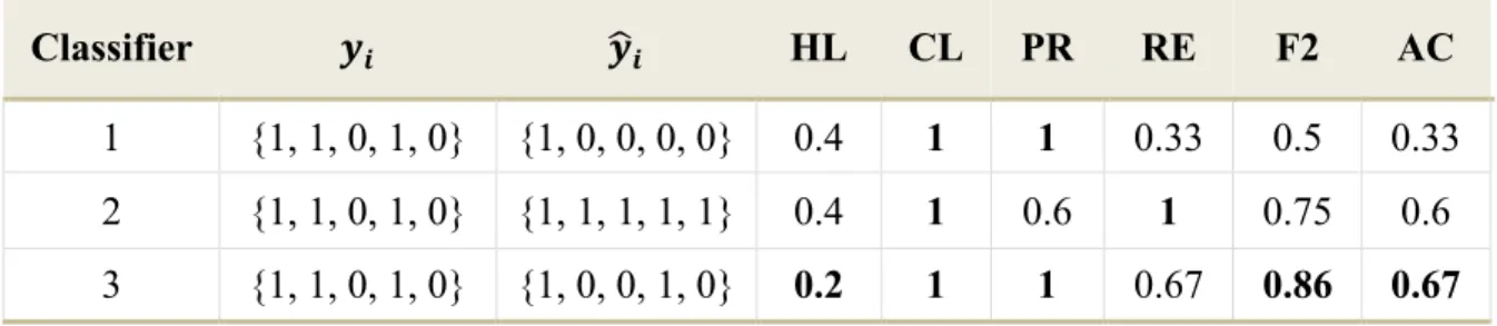
12 To illustrate the abovementioned measures, consider the vectors of true and predicted labels based on using three different classifiers, as given in Table 2.3. All measures except for HL are to be maximised, and the bold values correspond to the best classifier for a given measure.

Table 2.3: Illustration of six ML evaluation measures for three scenarios.

Classifier 𝒚𝒊 𝒚𝒊 HL CL PR RE F2 AC 1 {1, 1, 0, 1, 0} {1, 0, 0, 0, 0} 0.4 1 1 0.33 0.5 0.33 2 {1, 1, 0, 1, 0} {1, 1, 1, 1, 1} 0.4 1 0.6 1 0.75 0.6 3 {1, 1, 0, 1, 0} {1, 0, 0, 1, 0} 0.2 1 1 0.67 0.86 0.67

Due to the presence of multiple measures, determining whether a classifier is better than others depends on which evaluation measure is considered. In Table 2.3, the inverse relationship between PR and RE can be observed by comparing classifiers 1 and 2. Classifier 1 resulted in the highest PR but lowest RE. Out of the two classifiers, classifier 2 had the higher values of RE, F2 and AC, and therefore could be considered better than classifier 1. Comparing these results with the measures for classifier 3, it is clear that the third classifier has the best values for the HL, PR, F2 and AC measures. Therefore classifier 3 performed overall the best, based on this simple example.

There is some room for interpretation when it comes to ML classifier evaluation, depending on the problem. For example, if the exact match of labels is of importance for a specific application, CL could be given a larger weight. For the purposes of this thesis, a combination of equally weighted measures was considered when comparing classifiers in experimental work. The following section describes some of the specific approaches to ML classification in more detail.

(25)

13

2.6 DIFFERENT APPROACHES TO MULTI-LABEL

CLASSIFICATION

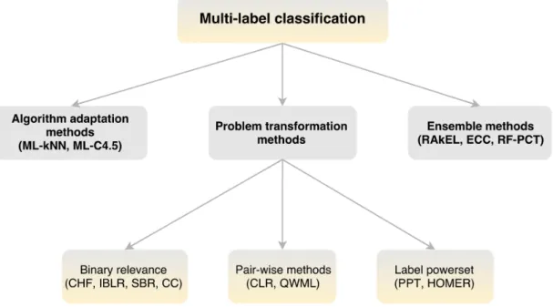
Classification in an ML context involves predicting more than one label for each observation. There are three main approaches to ML classification, namely the algorithm adaptation, problem transformation and ensemble approaches.

Algorithm adaptation (AA) approaches take a binary classification algorithm and adapt it for ML data to directly output multiple label predictions. Examples of this approach include the ML-kNN approach by Zhang and Zhou (2007), application of decision trees in the ML-C4.5 algorithm by Clare and King (2001), as well as AdaBoost.MH and AdaBoost.MR boosting algorithms by Schapire and Singer (2000). These approaches are algorithm-specific and can result in effective models. However, for some classifiers adapting the algorithm can be a complex task.

Problem transformation (PT) approaches involve adapting the data to the algorithm. These approaches transform the ML dataset into one or more binary datasets. The PT approaches use binary classification methods and transform predictions back to ML representations. One of the main advantages of this approach lies in using existing binary classification algorithms. Methods of transforming ML datasets include binary relevance, label powerset and pairwise methods (Madjarov et al., 2012). The PT approaches will be the primary focus of this thesis.

Ensemble approaches are extensions of the AA and PT methods. They usually consist of repeating a specific method numerous times in order to improve it. Examples include random k-labelsets (RAkEL) by Tsoumakas and Vlahavas (2007), ensembles of classifier chains by Read et al. (2011), and RF of predictive clustering trees (RF-PCT) by Kocev et al. (2007). These methods are computationally intensive and require further tuning of parameters, but can provide accurate models.

Apart from the traditional approaches to ML learning, research done in various fields contributed with alternative approaches to ML classification. For example, ML output coding uses the system of encoding labels into a lower-dimensional space, predicting encoded labels in this space and then decoding predictions back to the original label space. This scaling allows for simpler predictions and graphical

(26)

14 representations. ML output coding methods include principal label space transformations (Tai & Lin, 2012) and output coding with canonical correlation analysis (Zhang & Schneider, 2011). The following figure summarises some of the most significant approaches to ML classification. The PT approaches are described in more detail in the following section.

Figure 2.1: Summary of multi-label classification methods.

2.7 PROBEM TRANSFORMATION METHODS

2.7.1 BINARY RELEVANCE

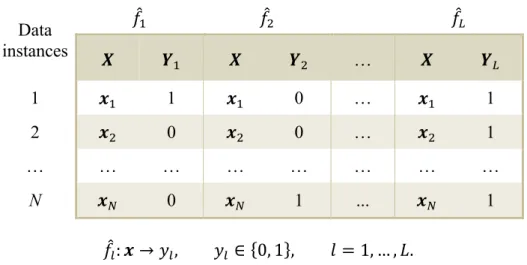
One of the best-known problem transformation approaches is known as binary relevance (BR). This method simply transforms the ML problem into L independent single-label binary problems. A binary classifier is then constructed for each of the L problems. These classifiers are responsible for predicting labels for the corresponding response variables. Table 2.4 summarises this approach.

Often the assumption of label independence is somewhat unrealistic. Consider for example music frequencies that can be associated with correlated music instruments. Ignoring this information may lead to inaccurate predictions of instruments that usually do not play together in practice, such as trumpet and harp. The BR classifier

(27)

15 focuses on marginal label distributions instead of joint distributions, thus ignoring label dependence altogether. On the other side, the strong independence assumption makes BR computationally efficient, simple and intuitive. Moreover, since BR treats the labels independently, it is not affected by a change in label dependence structure.

Table 2.4: Binary relevance method.

Data instances 𝑓_L 𝑓₎ 𝑓_N 𝑿 𝒀_L 𝑿 𝒀₎ … 𝑿 𝒀_N 1 𝒙_L 1 𝒙_L 0 … 𝒙_L 1 2 𝒙₎ 0 𝒙₎ 0 … 𝒙₎ 1 … … … … N 𝒙_T 0 𝒙_T 1 ... 𝒙_T 1 𝑓_s: 𝒙 → 𝑦_s, 𝑦_s ∈ 0, 1 , 𝑙 = 1, … , 𝐿.

The BR approach is referred to in almost every piece of literature on ML classification, and many methods use it as the foundation of their proposal. Examples include classification with heterogeneous features (Godbole & Sarawagi, 2004), instance-based logistic regression (Cheng & Hüllermeier, 2009), and classifier chains Read et al. (2011). In its original form, the BR method considers label dependency of first-order. The BR classifier ignores the label correlations, considering every label independently without regard for other labels.

2.7.2 LABEL POWERSET

In terms of modelling label dependence, label powerset (LP) (Tsoumakas & Vlahavas, 2007) lies on the opposite side compared to BR. Instead of splitting the label set according to the L separate labels, it joins all labels corresponding to a single case into one label class. Observations with the same label combination are labelled with the same label class. The new single label classes are therefore no longer binary but multi-class. The ML classification problem is thus transformed into a multi-class problem. Following the transformation, classification is performed using appropriate multi-class classifiers. The LP transformation is represented in the following table:

(28)

16 Table 2.5: Label powerset method.

Data instances Predictors Labels 𝑿L 𝑿) … 𝑿P Y 1 𝑥_LL 𝑥_L) … 𝑥_LP 1 2 𝑥_)L 𝑥₎₎ … 𝑥_)P 1 … … … … N 𝑥_TL 𝑥_T) … 𝑥_TP 3 𝑓: 𝒙 → 𝑦, 𝑦 ∈ 1,2, … , 𝐾 , 𝐾 ≥ 2.

This intuitive and easy transformation leads to a few desirable properties. Whereas the BR approach ignores the label dependence completely, the LP approach considers the full conditional joint distribution of the labels. This is as a result of the label structure left untouched during the transformation phase.

The LP approach also has some disadvantages. Maintaining the structure comes at a price of having a large number of label classes as the number of label combinations increases. A large number of classes make multi-class classifiers computationally inefficient. Furthermore, there is typically an imbalanced distribution of label classes. Label combinations with low frequencies contribute to this imbalance. The predictions based on an imbalanced distribution are more challenging, as there are few data points for the infrequent label combinations to use. Lastly, any label combination that is not modelled at the training phase will not be considered for prediction, resulting in model bias. These limitations of LP can make multi-class classification very difficult.

Pruned problem transformation (PPT) (Read, 2008) is an extension of the LP method that initially transforms the ML dataset in the same way as LP. Most of the issues identified for the LP method are caused by having a large number of class labels. PPT aims at reducing the number of classes by eliminating the most infrequent ones. Furthermore, PPT provides simpler models than LP and focuses on the most important label combinations. It is a computationally more efficient process, potentially without class imbalance issues. However, bias increases as fewer label

(29)

17 combinations are considered for prediction. On the other hand, PPT requires specifying a threshold that determines which label combinations are considered infrequent. It is also important to note that by removing the infrequent observations the training dataset becomes smaller, with less information entering the model. Despite these issues, a PPT model can be useful for situations where only the most frequent label combinations are of interest.

Other modifications of the LP method include an ensemble approach, RAkEL, and hierarchy of ML classifiers (HOMER) (Tsoumakas et al., 2008), where labels are first clustered and a classifier is constructed for each cluster of labels. In general, LP approaches consider label dependency of higher-order. Specifically, the transformation implemented in LP approaches allows for consideration of the influences between all labels.

2.7.3 PAIRWISE METHODS

Pairwise methods are another PT approach to ML classification (Hüllermeier et al., 2008). These methods try to capture a second-order label dependency by considering every label pair in a dataset. Pairwise methods consider the interaction between all pairs of labels. The idea is to transform the dataset of L labels into N(NuL)

) datasets, one for each label pair. Each of these datasets contains a set of binary labels (𝑦_Z, 𝑦_a, 𝑗 ≠ 𝑘) with the corresponding observations. The task is thus simplified to using a binary classification technique. The pairwise method is summarised in the following table:

Table 2.6: Pairwise method. Data instances 𝑓_L 𝑓₎ 𝑓N(NuL) ) 𝑿 𝒀_𝟏 𝒗𝒔. 𝒀_𝟐 X 𝒀_𝟏 𝒗𝒔. 𝒀_𝟑 … X 𝒀_𝑳u𝟏 𝒗𝒔. 𝒀_𝑳 1 𝒙L 1 𝒙L 0 … 𝒙L 1 2 𝒙₎ 0 𝒙₎ 0 … 𝒙₎ 1 … … … … N 𝒙_T 0 𝒙_T 1 ... 𝒙_T 1

(30)

18 At prediction time each of the N(NuL)₎ binary classifiers predicts a label for a new case and the predicted label receives a vote. These votes are aggregated over all classifiers and ranked. The final set of predicted labels are the 𝑀_~• labels with the most votes. The parameter 𝑀_~• can be specified or determined from the data. Alternatively, a method called calibrated label ranking (Fürnkranz et al., 2008) makes use of an artificially created label that acts as a threshold. Other adaptations of the pairwise method include the QWeighted method proposed by Mencía et al. (2010).

Some of the aspects of pairwise learning include computational considerations and label dependency. The number of classifiers that need to be constructed can be significantly more than that of BR, for N(NuL)₎ > 𝐿. However, the number of observations for each classifier is not constant and can be lower than in BR. Only the cases that are labelled with either of the pair of labels considered are included in each of the classifiers. Some of the classifiers will therefore have more data cases to learn from. Lastly, pairwise methods consider only a second-order dependency. The question arises whether it is a sufficient representation of the truelabel relationship. Some of the most significant methods for ML classification were summarised in this section. Which of these methods performs the best and which should be used in practical applications? It is important to note that just as with binary classification, the best method for ML datasets in general does not exist. However, it could be claimed that RF and boosting are very popular and accurate binary classifiers. Similarly in an ML setting, decision tree-based models are efficient and fast, PT methods that are BR-based are flexible and ensemble methods have strong predictive performance (Read, 2013). According to an extensive study done by Madjarov et al. (2012), overall the best methods were RF-PCT, HOMER and then BR and CC. It is however very important to note that these results, as well as any other results reported in the literature are based on numerous evaluation measures, which tend to favour different approaches. It is therefore not as straightforward to evaluate an ML classifier, as it is to evaluate a binary classifier, as discussed in Section 2.5. The following chapter focuses on a specific PT approach, classifier chains, as well as its limitations and modifications. The proposed ML classifier is also described in this chapter.

(31)

19

CHAPTER 3: Classifier chains in multi-label

classification

3.1 CLASSIFIER CHAINS

Classifier chains (CC) were introduced by Read et al. (2011). This approach is derived from the BR method. It assumes that conditional label dependence exists and uses the idea of chaining to exploit the label dependence information. The key idea is to capture some of these dependencies, while keeping the process computationally efficient. CC aim at finding a compromise between ignoring the label dependence completely and estimating the complex joint conditional distribution.

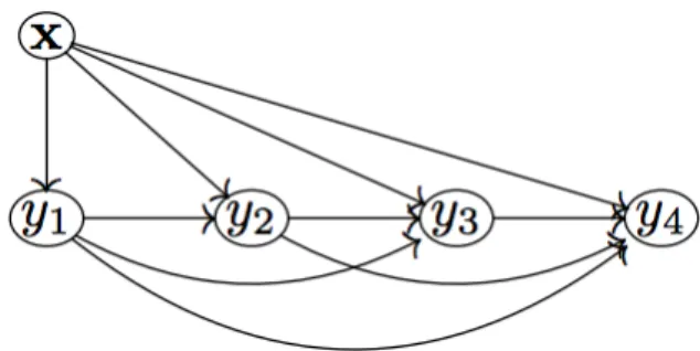
In its original formulation, CC construct a single chain of L classifiers, each predicting a corresponding label. The chaining is illustrated in Figure 3.1. In this figure, the first classifier involves predicting Y1 using only information from X. The second label is predicted from both X and Y1 via the second classifier. This process is repeated L times, resulting in L classifiers. What makes this process different from BR is an expanding feature space for each link in the sequence. At each consecutive chain link, the feature space gets appended with the true binary label from the previous link.

Figure 3.1: Illustration of the CC training algorithm with four chain links (Read, 2013).

The original CC algorithm is as follows: For 𝑖 = 1, 2, … , 𝐿:

1. Fit a base classifier 𝑓_Q(.) using 𝑋_L, 𝑋₎, … , 𝑋_P‚QuL and 𝑌_Q as training data. 2. Extend the training data by a new variable 𝑋_P‚Q, containing the true labels 𝑌_Q.

(32)

20 Consider a new case with input vector 𝒙₄. : 𝑃×1. In order to classify new cases, the following steps are required:

1. Compute 𝑌_L(𝒙₄) using only the predictors in 𝒙₄.

2. Append 𝑌_L(𝒙₄)to 𝒙₄and use this augmented vector to compute 𝑌₎(𝒙₄).

3. Repeat Step 2 for every label until all labels are predicted. The last label is predicted using the feature vector [x0, 𝑌_L 𝒙₄ , …, 𝑌_NuL(𝒙₄)].

The method of classifier chains enjoys some of the advantages of the BR method, including low memory requirements and computational efficiency. Similar to BR, it requires construction of L classifiers but the feature space is larger along the chain. Moreover, CC makes use of the chaining method and can take label correlations into account. However, it is important to note that it does not manage to model the full joint conditional distribution 𝑃 𝒀 𝑿 , since it only considers marginal label distributions in a chain-wise manner. The first label in the chain is modelled and predicted without taking any other labels into account, whereas the last label in the chain gets information from all the other labels. Despite this simplification of the underlying relationship, the CC method managed to outperform BR in various studies, including a paper by Read et al. (2011).

Interesting questions regarding the original idea of classifier chains arise. Firstly, during the training phase the feature vector is appended with true labels, whereas in the test phase it is expanded with predicted labels. This adds an additional layer of complexity as the classifier relies on accurate predictions of previous labels at the test phase. Should the feature space be expanded with incorrectly classified labels, propagation of error down the chain results. Ideally, such predictors should not be included in the subsequent models. The original CC does not account for a possibility of such error.

Secondly, the conditional label dependence is estimated using the sequence in which the labels enter the chain. In a CC classifier the order is random, starting with the first and ending with the last label. Therefore, the last label in the chain can make use of information from all the other labels. A question arises whether a random chain sequence should be used. It is generally expected that some labels would be more significant in explaining the remaining labels than others. The following experiment

(33)

21 was done in order to see whether the label sequence order has an effect on the accuracy of the classifier.

The analysis was conducted using the emotions dataset, consisting of six labels and 72 predictors. A more detailed description of the emotions dataset is provided in Section 5.2. The dataset was split into training and a test set using 75% and 25% of the data respectively. There were in total 6! = 720 label permutations of interest. For every label permutation, the CC classifier was fitted to the training dataset, using RF of 200 trees as the base classifier, and label sequence 𝒋Q, 𝑖 = 1, … ,720. For example,

𝒋_Q = (1, 2, 3, 4, 5, 6) would indicate that the original CC classifier was implemented.

The RF classifier is described in more detail in Section 4.5.3.

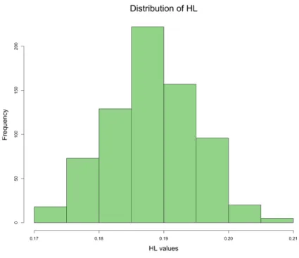
After the fitting process, the test set was predicted using the CC model, and a HL measure was computed for each repetition. This measure was chosen randomly, and its purpose was to be an indication of possible differences in performance for the different label sequences. Figure 3.2 shows distribution of HL based on the 720 models using label sequences 𝒋_Q, 𝑖 = 1, … , 720. The R code of this analysis is provided in Appendix A.1.

(34)

22 The HL distribution is fairly symmetric and slightly skewed to the right. These results are indicative of the effect of the different label sequences. The figure shows that some label orderings performed better than others in terms of HL. However, it is not correct to say that label sequence that provided the lowest value of HL is the best sequence for the emotions dataset in general. Due to data variability, a different training/test split is likely going to provide another ‘best’ label sequence. Furthermore, HL is just one approach for evaluating ML classifiers. It is always good practice to consider other evaluation measures, in order to obtain a more robust evaluation.

The idea of having a non-random label sequence order has also been explored in Cheng et al. (2010). In practice, it is not plausible to fit a classifier to a large dataset using all label permutations in order to choose the best label sequence. However, there have been numerous modifications of CC, which will be discussed in the next section.

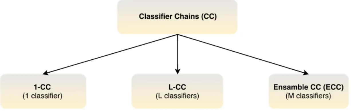
3.2 MODIFICATIONS OF CLASSIFIER CHAINS

Since its introduction, CC received a lot of attention in statistical research, including various modifications and implementations. The number of published papers that at least marginally deal with CC is surprising. Most of these methods are inspired by the original chaining idea and address some of its characteristics, shortcomings or propose a new approach altogether. Research is not limited to statistical literature, but includes areas of machine learning, computer science and genetics, with various interesting practical applications. The majority of papers explore the idea of estimating conditional label dependence and selecting the label sequence in the chaining process.

To introduce some of the modifications of the CC algorithm, the following notation is used. Let 𝜉 denote the set of all possible permutations of the integers 1, 2, … , 𝐿, and write 𝒋 for a permutation from this set. The elements of 𝒋 are denoted by 𝑗_L, 𝑗₎, … , 𝑗_N . The original CC procedure implements L binary classifiers using the permutation 𝒋 = 1, 2, … , 𝐿 . The 𝑙c‰_{of these classifiers is trained on the input data}

(35)

23 𝒙, 𝒚_L, … , 𝒚_suL , using 𝒚_s as the response, for 𝑙 = 1, 2, … , 𝐿. Here, for 𝑙 = 1, the input data is simply x.

3.2.1 ENSEMBLE OF CLASSIFIER CHAINS

The CC authors (Read et al., 2011) proposed an alternative algorithm called ensemble classifier chains (ECC). In ECC, M permutations 𝒋_L, 𝒋₎, … , 𝒋_Š are randomly selected from 𝜉 and ordinary CC are trained using each of these permutations to identify a label sequence. Only a random subset of the training data is used for every classifier. In the empirical work done in Read et al. (2011), a subset of 67% of the data was used as the training data for every classifier. Each of the M CC classifiers assigns a label vector, 𝒚‹ 𝒙 , to a new data case with input vector x, 𝑚 = 1, … , 𝑀. The final assignment of labels to x requires specification of a threshold, say t, where

1 ≤ 𝑡 ≤ 𝑀 . According to the ECC approach, 𝑦_s 𝒙 = 1 if and only if the

𝑙c‰ _{component of} _𝒚 ‹ 𝒙 Š

‹SL is greater than or equal to t. The ECC thus implements a thresholded voting system, where each of the M classifiers votes for the labels it predicts.

Although ECC are intuitively sound, perform well (Read et al., 2011) and use a more robust way of working with the chain sequencing, they are computationally expensive. Not only do they require more classifiers to be computed, but values for the number of models M, as well as the threshold t need to be specified or determined from the data.

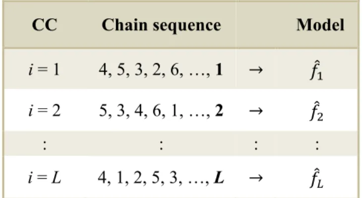
3.2.2 1-CLASSIFIER CHAINS

Both CC and ECC use random label sequences and therefore do not explicitly use the existing label dependence structure. This issue gave rise to another way of seeing CC. What if the label sequence could be selected non-randomly to capture the label dependencies more accurately? This sequence could be determined data dependently. Using data to define the best sequence would require a definition of what ‘best’ means: best in terms of one of the ML evaluation measures, or a combination of all of the measures? Approaches to identifying a single label sequence result in classifiers

(36)

24 that are based on a non-random label sequence. Let us refer to these as ‘1-CC’ classifiers.

In the 1-CC approach a single permutation 𝒋 from 𝜉 is used to identify the sequence in which label vectors are appended to the input matrix. However, now 𝒋 is not selected randomly, but determined in some way from the training data. A first possibility in this regard considers only the label data. For example, let 𝑟_QZ denote the correlation between 𝒚_Q and 𝒚_Z, 𝑖, 𝑗 = 1, … , 𝐿; 𝑖 ≠ 𝑗. Compute 𝑟_s = _NuLL _Z•s 𝑟_sZ for

𝑙 = 1, … , 𝐿, the average absolute correlation between 𝒚_s and all the other label

vectors. Suppose 𝑟_s_• < 𝑟_s_’ < ⋯ < 𝑟_s_`. Then the permutation used according to this approach could be defined by 𝒋 = 𝑙_L, 𝑙₎, … , 𝑙_N . The label that corresponds to the highest average absolute correlation with all other labels is considered last for prediction. This way the most correlated label can use the information from the other labels and learn from them at the training stage.

More generally, the selection of permutation 𝒋 for the 1-CC classifiers can be done by:

1. Using only the label variables:

1.1. Absolute correlation

The permutation j is computed as described above.

1.2. RF importance values

Let 𝛪_QZ denote the Gini importance value between 𝒚_Q and 𝒚_Z, 𝑖, 𝑗 = 1, … , 𝐿; 𝑖 ≠ 𝑗, obtained from fitting a RF model to 𝒚_Q using all other labels as predictors. The Gini measure is described in more detail in Section 4.5.3. Compute 𝐼_s = L

NuL Z•s𝐼sZ for 𝑙 = 1, … , 𝐿, the average contribution of all other labels for label 𝑙. Suppose 𝐼_s_• < 𝐼_s_’ < ⋯ < 𝐼_s_`, then the permutation is 𝒋 = 𝑙_L, 𝑙₎, … , 𝑙_N .

(37)

25

1.3. ReliefF

Let 𝑟𝐹_QZ denote the ReliefF value between 𝒚_Q and 𝒚_Z, 𝑖, 𝑗 = 1, … , 𝐿; 𝑖 ≠ 𝑗. ReliefF is a multivariate measure of relationship between predictors and a label that takes into account the interaction between predictors. A predictor receives a high value of 𝑟𝐹 if its values differ for examples from different classes, and gets penalised with a low 𝑟𝐹 value if its values are different for examples from the same classes (Spolaôr et al., 2013). Compute 𝑟𝐹_s = _NuLL _Z•s𝑟𝐹_sZ for 𝑙 = 1, … , 𝐿, the average contribution of all other labels for label 𝑙. Suppose 𝑟𝐹_s_• < 𝑟𝐹_s_’ < ⋯ < 𝑟𝐹_s_`, then the permutation is 𝒋 = 𝑙_L, 𝑙₎, … , 𝑙_N .

2. Using both input and label variables:

2.1. Ordered CC (Keikha & Hashemi, 2016)

Consider an ML dataset split into training and test sets. Using the BR approach, fit 𝒚_s using the training data with RF as the base classifier, for 𝑙 = 1, … , 𝐿. Predict the corresponding labels for the test dataset, using the fitted BR model. Let 𝑦_Qs be the predicted value for the 𝑖c‰_{observation and}_𝑙c‰_{label. Compute the accuracy measure} of each of the label predictions, defined as 𝐴𝐶_s =_TL T 𝐼 𝑦_Qs = 𝑦_Qs , 𝑙 = 1, … , 𝐿.

QSL

Suppose 𝐴𝐶_s_• > 𝐴𝐶_s_’ > ⋯ > 𝐴𝐶_s_`, then the 1-CC permutation is 𝒋 = 𝑙_L, 𝑙₎, … , 𝑙_N . The idea is to place the labels that are most likely to be correctly predicted first, so that the subsequent labels can make use of correctly predicted labels.

2.2. Canonical correlation analysis (CCA)

Consider a CCA between 𝒙 = 𝒙_L, 𝒙₎, … , 𝒙_P and 𝒚 = 𝒚_L, 𝒚₎, … , 𝒚_N resulting in the vectors of canonical coefficients a, bthat maximise the canonical correlation 𝜌 =

𝑐𝑜𝑟𝑟 𝒂™_{𝒙, 𝒃}™_{𝒚 .}_{The coefficient 𝑏}

𝒍 represents the strength of label l in relation to 𝒙. Suppose 𝑏_s_• > 𝑏_s_’ > ⋯ > 𝑏_s_`, then the permutation is 𝒋 = 𝑙_L, 𝑙₎, … , 𝑙_N , so that the label that has the strongest relationship with the features would be first in the sequence and likely be predicted most accurately by the CC.

(38)

26 In Section 3.1 it was stated that the order of the labels in the label sequence of CC does have an impact on the ML evaluation measures. In the following analysis, the use of a 1-CC classifier with a non-random label sequence was compared to the BR and CC classifiers, in order to see whether the 1-CC approach resulted in better performance. An experiment was conducted, in which the BR, CC as well as the five 1-CC methods were used for ML classification of the emotions dataset. All of the classifiers used RF of 200 trees as the base classifier. The analysis was repeated using 30 random dataset training and test splits. All of the classifiers were fitted on the same data splits. The means and standard deviations of six ML evaluation measures, defined in Section 2.5, were computed for each of the classifiers. The results are summarized in Table 3.1, and the corresponding R code is provided in Appendix A.2. All measures except for HL were to be maximised, and the bold value indicates the best classifier for a specific ML measure.

Some of the 1-CC methods performed slightly better than others in terms of the individual evaluation measures. The original CC performed better compared to BR for HL, CL, RE, F2 and AC. The 1-CC methods performed better than CC in terms of CL, RE, F2 and AC, but not for HL and PR. The 1-CC classifier that implemented the CCA method to identify the label sequence did overall consistently well compared to the other 1-CC methods. However, the performance differences based on all measures were relatively small, and further analysis would be necessary to determine whether the differences were significant.

These findings make intuitive sense, as both CC and 1-CC methods make use of the chain structure, whereas BR treats the labels independently. However, using only a single label sequence may not be sufficient for capturing information from the joint conditional distribution of labels. This could explain the relatively small differences amongst the CC and 1-CC methods. The five 1-CC methods summarised above are just a few examples of how a single label sequence method could be applied. All of them identify the best label sequence based on the characteristics of the dataset, prior to fitting an ML classifier.

(39)

27 Table 3.1: ML classification of the emotions dataset using the BR, CC and 1-CC

algorithms. Mean HL CL PR RE F2 AC BR 0.182 0.313 0.758 0.619 0.681 0.541 CC 0.181 0.322 0.746 0.642 0.690 0.559 𝑪𝑪_𝒄𝒐𝒓 0.182 0.324 0.743 0.642 0.689 0.560 𝑪𝑪𝒓𝒇𝒊𝒎𝒑 0.182 0.320 0.743 0.641 0.688 0.558 𝑪𝑪_{𝒓𝒆𝒍𝒊𝒆𝒇𝒇} 0.182 0.329 0.735 0.650 0.690 0.562 𝑪𝑪_𝒐𝒄𝒄 0.183 0.330 0.730 0.646 0.686 0.561 𝑪𝑪_{𝒄𝒂𝒏𝒄𝒐𝒓} 0.181 0.334 0.738 0.650 0.691 0.565 Std. Dev. HL CL PR RE F2 AC BR 0.014 0.034 0.029 0.027 0.026 0.027 CC 0.015 0.038 0.031 0.030 0.029 0.030 𝑪𝑪_𝒄𝒐𝒓 0.015 0.032 0.030 0.033 0.030 0.031 𝑪𝑪_{𝒓𝒇𝒊𝒎𝒑} 0.016 0.042 0.031 0.032 0.030 0.033 𝑪𝑪_{𝒓𝒆𝒍𝒊𝒆𝒇𝒇} 0.015 0.035 0.029 0.029 0.027 0.030 𝑪𝑪_𝒐𝒄𝒄 0.016 0.036 0.033 0.034 0.031 0.034 𝑪𝑪𝒄𝒂𝒏𝒄𝒐𝒓 0.015 0.034 0.032 0.030 0.029 0.030

Another way of determining the best label sequence is by fitting the 1-CC classifier for all permutations of the label sequence, and testing which sequence performs best. In general, one could use K-fold cross validation (K-CV) to determine the best label sequence from the data in the following way. Let the tuning parameter 𝜃 denote a label sequence, and let 𝜃_Q be all the permutations of interest, 𝑖 = 1, … , 𝐿!. The dataset is split into K random non-overlapping partitions. Using the 𝑘c‰_{partition as the test} set, the 1-CC classifier using 𝜃_L is fitted to the other K-1 partitions. The classifier’s