http://www.aimspress.com/journal/MBE DOI: 10.3934/mbe.2019391 Received: 22 May 2019 Accepted: 30 July 2019 Published: 26 August 2019 Research article
FRS: A simple knowledge graph embedding model for entity prediction
Lifang Wang1, Xinyu Lu1, Zejun Jiang1,∗, Zhikai Zhang1, Ronghan Li1, Meng Zhao1and Daqing Chen2
1 School of Computer Science and Engineering, Northwestern Polytechnical University, Xi’an,
710072, PR China
2 Division of Computer Science and Informatics, School of Engineering, London South Bank
University, London SE1 0AA, UK
* Correspondence: Email: [email protected]
Abstract: Entity prediction is the task of predicting a missing entity that has a specific relation-ship with another given entity. Researchers usually use knowledge graphs embedding(KGE) methods to embed triples into continuous vectors for computation and perform the tasks of entity prediction. However, KGE models tend to use simple operations to refactor entities and relationships, resulting in
insufficient interaction of components of knowledge graphs (KGs), thus limiting the performance of the
entity prediction model. In this paper, we propose a new entity prediction model called FRS(Feature
Refactoring Scoring) to alleviate the problem of insufficient interaction and solve information
incom-pleteness problems in the KGs. Different from the traditional KGE methods of directly using simple
operations, the FRS model innovatively provides the procedure of feature processing in the entity prediction tasks, realizing the alignment of entities and relationships in the same feature space and improving the performance of entity prediction model. Although FRS is a simple three-layer network, we find that our own model outperforms state-of-the-art KGC methods in FB15K and WN18. Through
extensive experiments on FRS, we discover several insights. For example, the effect of embedding size
and negative candidate sampling probability on experimental results is in reverse.
Keywords: knowledge graphs; entity prediction; knowledge graphs embedding; FRS
1. Introduction
Nowadays, we receive a variety of information every day. How to make better use of information that changes so quickly is something we deserve to think about. The development of computer science technology has promoted the popularity of knowledge graphs (KGs) [1–3], which is a semantic network [4] that reveals and describes the relationships between entities in the real world. In this paper, a
knowledge graph means triples. Entities are the most basic elements in a KG, and different entities may have different relationships. Let E represent a set of entities, R represent a set of relationships between entities. A knowledge graph can be expressed as a collection of a number of triples:
KG = {(h,r,t)|h,t∈E,r ∈R} (1.1)
where h represents the head entity, t represents the tail entity, and r denotes the relationship which
is used to connect the head entity and the tail entity, i.e.,< Obama,Place o f Birth,Honolulu >. In essence, KGs are multi-relational graphs composed of entities (nodes) and relationships(edges). Each edge consists of a head entity, a relationship, and a tail entity. The graph structures and large volume often make KGs useful for regular users to access valuable information. There are many widely used knowledge bases on the Internet, such as Freebase [5], Wikidata [6] and DBpedia [7]. When applying knowledge graphs to a natural language task, the correctness and coverage determine its contributions to the task. Common natural language processing (NLP) [8] tasks, such as Question-answering systems and information retrieval tasks, often require a KGs system as support. However, tasks based on
KGs are often affected by incompleteness. Incompleteness in this paper means that a triple misses an
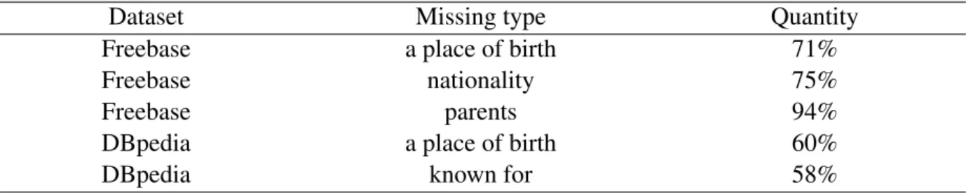
entity or a relationship. Therefore, it is necessary to study Knowledge Graph Completion (KGC) [9– 11] methods to complete missing information with the purpose of improving the quality of KGs and the performance of real-world applications. KGC methods mainly use structured knowledge to infer factual information which is already covered in a KG. Table 1 shows that even the ultra-large-scale knowledge graphs still lack a lot of important information.
Table 1. Statistics of missing type and quantity.
Dataset Missing type Quantity
Freebase a place of birth 71%
Freebase nationality 75%
Freebase parents 94%
DBpedia a place of birth 60%
DBpedia known for 58%
In general, KGC tasks can be divided into two subtasks: Link prediction [12] and Entity predic-tion [13]. Link predicpredic-tion aims to automatically complete the missing relapredic-tionships in the knowledge graphs. Entity prediction aims to automatically complete the missing entities in the knowledge graphs. This article focuses on entity prediction tasks. The benefit of knowledge graphs embedding(KGE) [14] methods in a variety of practical applications stimulates us to explore its promising use in solving the KGC problems. Extensive research [15] has been done on KGC to fill in missing entities or relation-ships by KGE methods. The KGE methods embed the entities and relationrelation-ships of the knowledge graphs into the continuous vector space and then complete some downstream KGs applications such as KGC. Most existing KGE technologies perform entity prediction tasks based on observed facts. An entity prediction task based on the KGE method first represents the entity and the relationship as the form of the vectors, i.e., the real value vectors, and then defines the scoring function to measure the plausibility of triples. The ultimate goal is to maximize the total plausibility of triples. The embedding vectors of entities and relationships are used for the interaction of components of given triples. Taking
the model ProjE [16] as an example, before using the scoring function, the model simply uses diagonal matrices to combine entities and relationships. The refactoring formula is as follows:
e⊕r=Dee+Drr (1.2)
whereDe andDrare the specific matrix combination operators. This combination method ignores the
interaction between entities and relationships in the same embedding space, resulting in insufficient
interaction. To bridge this gap, we explore how to handle the problem of insufficient interaction and
use a simple and efficient neural network to perform KGC tasks.
Inspired by the above observations, this paper proposes a new entity prediction model called FRS(Feature Refactoring Scoring) based on the idea of shared parameters and knowledge graphs em-bedding. The main characteristics of the proposed approach are:
1. Instead of requiring a prerequisite or a pretraining process, FRS is a self-sufficient model over
the length-1 relationship and doesn’t occupy expensive multi-hop paths through the knowledge graphs.
2. FRS innovatively introduces feature engineering methods in the knowledge graphs completion models. In the feature processing layer, the alignment between entities and relationships in the same feature space is realized by using the idea of shared parameters neural network. The experi-ment proves that the feature processing layer alleviates the problem of insufficient interaction and provides a new idea for the KGC task.
3. Through extensive experiments of FRS, we find that the effect of embedding size and negative
candidate sampling probability on experimental results is in reverse. It contributes to the entity predictive model’s fine-tuning work.
4. Unlike the entity prediction model with complex networks, FRS can be regarded as a simple three-layer neural network entity prediction and outperforms state-of-the-art KGC methods.
2. Related works
This section introduces some of the basic concepts, definitions, and a few abbreviations in this article. In addition, we review different types of entity prediction algorithms and their score functions. 2.1. Background
Notations: Throughout this paper, we use uppercase bold letters to represent matrices(e.g.,M,W) and lowercase bold letters to represent vectors(e.g.,h,r,t). kxk1/2denotes either the`1norm or`2norm.
Let tanh(x) the hyperbolic tangent function, and sigmoid(x) the sigmoid function. The score function is used to measure the triples plausibility.
Definition 1. (Knowledge Graphs Embedding): a method of knowledge representation learning which embeds entities and relationships of knowledge graphs into continuous vector spaces.
Definition 2. (Entity Prediction): given two < r,t > or < h,r > as input, we consider the entity prediction as a ranking scoring problem where the top-k candidates in the scoring list are prediction results. The output list should follow the rules in this task, when outputting any two tail entitiesei,ej,
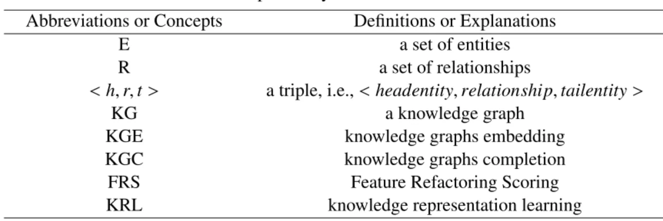
We summarize the mentioned abbreviations and concepts in this paper in Table 2.
Table 2. The important symbols and their definitions.
Abbreviations or Concepts Definitions or Explanations
E a set of entities
R a set of relationships
<h,r,t> a triple, i.e.,<headentity,relationship,tailentity>
KG a knowledge graph
KGE knowledge graphs embedding
KGC knowledge graphs completion
FRS Feature Refactoring Scoring
KRL knowledge representation learning
Entity prediction algorithms can be categorized into distance models and similarity matching mod-els. The main difference is that different models use different scoring functions. The distance model uses a distance-based scoring function, while the similarity matching model uses a similarity-based semantic matching scoring function.
2.2. Distance models
The distance model usually uses a distance-based scoring function to measure the probability of triples. Unstructured model (UM) [17] and structured embedding (SE) [18] are early stage models. Their structure is simple and can achieve good prediction results.
UM [17] treats triples with only a single relationship and all relationships set to zero vectorsr= 0. so the scoring function is
fr(h,t)= −kh−tk22 (2.1)
The model is simple and easy to expand, however, this method does not distinguish well between
different relationships in KGs. In order to solve this problem, SE [18] learns relationships specific
matrices for entities. The score function can be defined as: fr(h,t)= − Mr,1h−Mr,2t 1 (2.2)
where specific matrices Mr,1,Mr,2 ∈ Rd×d. The SE transforms vectors h and t of entities through
the corresponding specific matrices of the relationships r and then measures their similarity in the
transformation space, which reflects the semantic correlation of the head entities to tail entities in the relationship space. The SE model has a significant drawback: it uses two different matrices for the head and tail entities to project, and the coordination is poor. It is often impossible to accurately describe the semantic relationship between two entities and the relationship. Although the UM model and the SE model have a simple model structure, they have achieved good entity prediction results in the early stage, but they are not effective in the scenarios of the relationship directly related.
With the development of distributed representation, researchers find that word vectors sourcing from the word2vec [19] algorithm can capture invisible semantic information between words and words, as shown in the following:
vTokyo−vJapan ≈ vBerlin−vGermany (2.3)
Since the triple data has obvious relationship information, relationship r can be interpreted as the
translation of h to t. This is the main idea of the most representative distance model TransE [20].
TransE is inspired by translation invariance in the word vector space, where the relationship between
words usually corresponds to translations in potential feature spaces. TransE wants thath+r≈ twhen
measuring the plausibility of a triple. The score function can be defined as:
fr(h,t)=−kh+r−tk1/2 (2.4)
where fr(h,t) can be two options:L1−normorL2−norm. Compared with the previous models, TransE
has fewer parameters and low computational complexity, and can directly establish complex semantic relations between entities and relationships. However, due to the simplicity of TransE, it cannot handle complex relationships modelling. TransH [21] alleviates the problem of TransE in building complex
relationships. TransH projects h and t by a specific relationship matrix. The score function can be
defined as: fr(h,t)= h−w > rhwr+dr− t−w > rtwr 2 2 (2.5)
wherewr is the relationship specific hyperplane, dr is the relationship translation vector. These pro-posed models performed well for the one-to-many relationships. The TransH model makes entities have different representations of different relationships, and it simply assumes that entities and rela-tionships can be represented in a single semantic space. However, this simple assumption leads to inaccurate modeling of entities and relationships by TransH.
2.3. Similarity matching models
The similarity matching model usually uses a similarity-based semantic matching scoring function. They measure the plausibility of triples by matching the underlying semantic information of the entity and the relationships embodied in its vector space representation.
RESCAL [22] is based on three-dimensional tensor factorization. The scores function can be de-fined as follows:
s(h,r,t)= hMrt> (2.6)
whereMr is ak×krelationship matrix. RESCAL learns the embedding of entities and relationships
by minimizing the tensor reconstruction error and then completes the KGs using the scores of the reconstructed tensor. Neural Tensor Network(NTN) [23] replaces the linear transformation layer in traditional neural networks with bilinear tensors and links the head entities and tail entities vectors in different dimensions. The score function can be defined as:
fr(h,t)= u >
r tanh h >
Mrt+Mr,1h+Mr,2t+br (2.7)
whereMr ∈Rd×d×k denotes a tensor,Mr,1,Mr,2 ∈ Rk×d are weight matrices, and ur is the relationship
vector. NTN considers second-order correlation by introducing tensors to extend the single-layer neural network model. However, due to the parameter and the number of complexity of this model, it is
difficult to deal with large-scale KGs. ProjE [16] is designed to fill the missing information in KGs by a shared variable neural network. They reported that ProjE has a small parameter size and performs well on standard datasets. ProjE defines its function as:
h(e,r)= sigmoidWctanh(e⊕r)+bp
(2.8)
whereWc is the candidate matrix.
e⊕r= Dee+Drr+bc (2.9)
whereDe andDrare diagonal matrices. However, the enough feature processing for the triple data is
overlooked before using specific matrix combination operators. SENN [24] integrates the prediction tasks of head entities, relationships and tail entities into a neural network-based framework. The score function ofhead pred(r,t) is defined as:
s(r,t)=vhA
>
E
= f f · · · f [r;t]Wh,1+bh,1· · ·Wh,n+bh,nA>E
(2.10)
where f is an activate function, n represents the number of neural network layers, W is the weight
matrices, and b is the bias item. The result of relation prediction and entity prediction is improved.
However, based on a given triple, SENN needs to calculate the head entity prediction label vector and the tail entity prediction label vector separately, which is more complicated than the traditional model that only uses a single prediction label vector to complete the entity prediction task.
3. Problem statement
The similarity matching models tend to use simple matrix operators to combine entities and
rela-tionships, which is effective, and existing models such as ProjE [16] and RESCAL [22] can be proved.
However, the importance of feature processing for the triple data is overlooked. Feature processing is mainly used to enhance the interaction between triples, i.e., entities and entities, relationships and relationships, entities and relationships. Since the similarity matching model is based on the potential semantic similarity, the interaction between the triple data is the key of the entity prediction model. The interaction of this paper relies on feature engineering. There are usually two methods for feature engineering: one is manual processing, which requires more human intervention, and requires a deep understanding of the tasks involved to build better features. This method is feasible, but for more complex tasks, it takes a lot of manpower and resources to construct the appropriate features. Another method is knowledge representation learning [25–27], which automatically learns new representations from the data directly through machine learning algorithms, and is able to learn the appropriate fea-tures based on specific tasks. In this paper, a variant of feedforward neural networks is used as a feature engineering method to alleviate the problem of insufficient interaction.
3.1. F network
We start with the basic feedforward network model, which has only one neuron. A feedforward neural network is a basic network in which all nodes are organized into successive layers, each node receiving input from nodes in the earlier layers. Given an input (xi), the output can be defined as:
y= f n X i=1 Wixi+b (3.1)
Where the parameterWi is used to fit the data, bis a bias term, and f is the activation function. In a
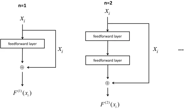
feedforward network, the chain structure is the interaction between layers, and the number of layers represents the depth of the network. This complex mapping can be seen as the interaction of feature information. Thus, we introduce a variant of the feedforward network, which is based on the shared pa-rameters and residual [28], specifically designed for feature representation of entities and relationships. The structure of the F network is shown in Figure 1.
feedforward layer i
x
⊕
ix
(1)( )
iF x
feedforward layer ix
⊕
(2)( )
iF
x
feedforward layer ix
n=1 n=2...
Figure 1. The structure of F network. Where nis the number of layers, xi is the input of F
network, andF(n)(x
i) is the output of F network.
Given the input (xi), the output of thenthlayerF(n)(xi) can be defined as:
F(n)(xi)=σ(F(xi)(n−1)W)+xi (3.2)
wherenis the number of layers,σdenotes that there is a mapping relation between the input data and
the shared parameterW, andxi is a residual item. According to the structure of Figure 3 and Equation
(3.2), we can get:
F(1)(xi)= f(xiW)+xi (3.3)
F(2)(xi)= f(f(xiW)W)+xi (3.4)
where f represents activation functions.The main identity of the F network is that it uses the idea of
4. Methodology
This section mainly introduces the details of the FRS model proposed in this paper and briefly gives the loss function and the negative sample sampling method.
4.1. Architecture
A typical entity prediction model usually consists of two steps:
step 1)Representation of entities and relationships.
step 2)Definition of similarity scoring function.
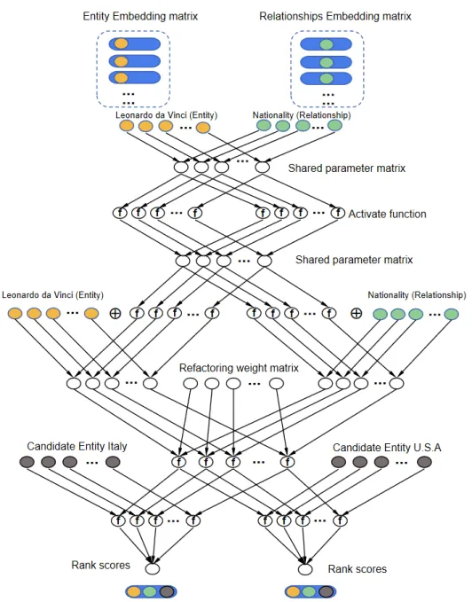
The first step is to embed entities and relationships into successive low-dimensional vector spaces. In the second step, the scoring function is to measure the plausibility of the triples. Based on the charac-teristics of the typical entity prediction model, this paper proposes a new neural network model where the entities and relationships are modeled by a three-layer structure with a feature processing layer, a refactoring layer, and a candidate prediction layer. The feature processing layer and the refactoring layer are used for the representation of entities and relationships, and then the candidate prediction layer is used for the measure of the similarity function. It is in line with the construction steps of a typ-ical entity prediction model. The explanation of FRS is as follows: given two embeddings as input, we consider the entity prediction as a ranking scoring problem where the top-k candidates in the scoring list are prediction results. To get this score list, we rank every possible candidate on a refactoring oper-ator defined by two input embeddings through the specific feature engineering method. Figure 2 takes the tail entity prediction task as an example. The input data is< LeonardodaVinci,Nationality,? >, and the candidate entities are< Italy > and< U.S.A >. The yellow nodes and brown nodes are row vectors, from the entity embedding matrix, and the green nodes are row vectors, from the relation-ships embedding matrix. It is worth noting that the three-layer network in this paper adopts the idea of shared parameters. Shared parameters are used in this paper to reduce training parameters and alleviate insufficient interaction.
4.1.1. Feature processing layer
Recent models have shown that specific matrix combination operators can refactor entities and relationships such as HoIE [29] and ProjE [16]. However, the importance of feature processing for the
triple data is overlooked before using specific matrix combination operators. Insufficient interaction
may limit the performance of the KGC model, so it is necessary to perform feature processing on the input data. To solve the insufficient interaction problem, the feature processing layer is proposed based on the F network. Intuitively, multi-layer F networks can more easily learn abstract and general feature information. As the training parameters increase layer by layer, we choose the two-layer F network as the feature processing layer. It can be defined as follows:
F(e)= f[f(eW)W]+e (4.1)
F(r)= f[f(rW)W]+r (4.2)
where f represents an activation function we use in training process,Wis ak×ksquare matrix which
represents feature processing weight. In this layer, entities and relationships share the same weight matrixW, while adding the residual itemseandr.
From the perspective of the interaction, entities and relationships are aligned by the shared
param-eterW. This alignment can be seen as some shared attributes that entities and relationships have after
passing through the same embedding space. The shared parameter Wcan be regarded as an
embed-ding space, and the entities and the relationships complete the interaction through the same embedembed-ding space. It can be summarized as the feature processing layer uses shared parameters to complete implicit interactions between entities and relationships.
4.1.2. Refactoring layer
The middle layer is the refactoring layer. Similar to most KGE models, this layer uses some specific matrix combination operators to combine entities and relationships. It can be defined as:
R(e,r)= [F(e)+F(r)]V (4.3)
whereVis ak×krefactoring weights matrix. The refactoring layer explicitly performs the interaction
between the entities and the relationships by the shared parameter. Explicit interaction refers to the use
of shared parameterVto refactor entities and relationships while completing the interaction.
4.1.3. Candidate prediction layer
The third layer is the candidate prediction layer, which is the output layer. The candidate prediction layer is based on the fact that the feature representation can capture the semantic similarity of triple data in the knowledge graphs. Therefore, by operating on the results of the output of the first two layers of the FRS, an embedding representation similar to the predicted result is obtained, and then, the similarity calculation is performed with the real candidate entities. We can define the candidate prediction process as:
S(e,r)= f[f(R(e,r))C+b] (4.4)
where C is a s×k candidate entities matrix, s denotes the number of candidate entities, k denotes
embedding size, f represents activation functions, and b is the candidate prediction bias. Since s
comes from the entity setE, and the FRS model structure is shared parameters, no additional variables
are needed. This layer obtains the final prediction results with a scoring list. 4.2. Sampling and loss function
In the algorithm of this paper, although the set of candidate entities does not increase the number of parameters because of entity variables sharing, if the model uses all the sets of entities to train each time, it will lead to a huge amount of computation. Therefore, the candidate sampling method should
be used to reduce the size of the candidate entity setC. We use the rules of word2vec [19] to sample
the candidate set negatively. It can be described as that the set of candidate entities used for training consists of a set of entities in all positive cases and a set of entities in a part of negative cases. We can simply use the binomial distributionB(1,Py) to indicate whether an entity in a negative instance is selected. Pyindicates the probability that the negative case is selected, and 1−Pyindicates the prob-ability that the negative case is not selected. To learn the representation of entities and relationships, we need a loss function to maximize the plausibility of triples. For a triple and a binary label vector,
Figure 2. FRS architecture for entity prediction. Take the tail entity prediction task as an example. The input is< LeonardodaVinci,Nationality,? >. The two tail candidate entities are< Italy > and< U.S.A >. The FRS model can be seen as a three-layer neural network structure with a feature processing layer, a refactoring layer, and a candidate prediction layer. The model finally outputs a list of scores of candidate entities. The yellow node represents the head entity, the green node represents the relationship, and the brown node represents the tail entity.
we can obtain the candidate prediction result from positive candidates and negative candidates. For all the entities, we apply a binary label vector to them which means entities inE−get 0 score and entities
inE+get 1 score. To fulfill the goal of maximizing the connection between the binary label vector and
candidate prediction results, we define the loss function in a similar way:
L(e,r,y)= − X i∈{i|yi=1} log (S(e,r)i)− X s Ej∼Pnlog(1−S(e,r)j) (4.5)
In the binary label vector,y ∈ C, yi = 1 indicates a positive lable; sdenotes the number of negative
samples originated from Ej∼Pn. According to all the settings, the ranking score of the i
th candidate entity is: S(e,r)i = sigmoid[tanh(R(e,r))C[i,:]+b] (4.6) R(e,r)= [F(e)+F(r)]V (4.7) F(e)= sigmoid[sigmoid(eW)W]+e (4.8) F(r)= sigmoid[sigmoid(rW)W]+r (4.9) 5. Experiments 5.1. Evaluation protocol
We use the following two evaluation metrics as the basis for the assessment: the average ranking of all correct entities (Mean Rank) and the correct entities that appear within the top-k elements (Hits@k). These two evaluation metrics are called Raw because the target prediction results are not considered in the evaluation process. If we take the target prediction results into consideration, these two evaluation metrics become Filtered. For example, when the input triple is< Italy,Contained by,?>and the target entity prediction result isT oscana. In the entity prediction task, we will get a top-2 list: Florenceand T oscana. The Raw Mean Rank and Hits@1 would be 2 and 0 respectively. The Filtered Mean Rank and the Filtered Hits@1 would both be 1. It only because the setting of Filtered ignores the other candidate entities although these are correct entities.
5.2. Experimental settings
For experiments with FRS, the omitted parameter settings of Adam are as follows: β1 =0.9, β2 =
0.999 and =1e−8. The number of epoch for all experiments in this paper is 100, and the initialization
of all parameters is derived from a normalized distributionUh−√6
k,
6
√ k
i
. We used the hyperparameter
settings are as follows: dropout probability pd =0.5, negative sampling probability pn =0.5,
embed-ding sizek=200, minibatchb=200. We manually set the learning rate change operator by using the
idea of learning rate decay in the process of model learning. The learning rate initial value is 0.01. 5.3. Results
This subsection will focus on the following three issues: First, what is the main similarity and
difference between the FRS and other KGC models? Second, how effective FRS is compared to other
contribution and limitation of the FRS model proposed in this paper? In the table, MR and FMR refer to Mean Rank and Filtered Mean Rank respectively. The capital letter F indicates the Filtered results. The two tables contain different models because the experimental results in this paper are all selected from the original papers. The original paper may only experiment with one dataset, either FB15K or WN18, and the results in the table strictly follow the results of the original paper. Table 3 shows the statistics of FB15K and WN18. Table 4 shows the evaluation results on FB15K. Table 5 shows the evaluation results on WN18.
Table 3.Statistics of the experimental datasets.
Dataset Entity Relationship Training Valid Test
FB15K 14951 1345 483142 50000 59071
WN18 40943 18 141442 5000 5000
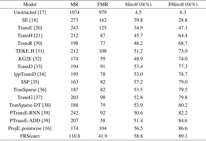
Table 4. Entity prediction results of different models on FB15K.
Model MR FMR Hits@10(%) FHits@10(%)
Unstructed [17] 1074 979 4.5 6.3 SE [18] 273 162 39.8 28.8 TransE [20] 243 125 34.9 47.1 TransH [21] 212 87 45.7 64.4 TransR [30] 198 77 48.2 68.7 TEKE H [31] 212 108 51.2 73.0 KG2E [32] 174 59 48.9 74.0 TransD [33] 194 91 53.4 77.3 lppTransD [34] 195 78 53.0 78.7 SSP [35] 163 82 57.2 79.0 TranSparse [36] 187 82 53.5 79.5 TransG [37] 203 98 52.8 79.8 TranSparse-DT [38] 188 79 53.9 80.2 PTransE-RNN [39] 242 92 50.6 82.2 PTransE-ADD [39] 207 58 51.4 84.6 ProjE pointwise [16] 174 104 56.5 86.6 FRS(our) 110.8 41.9 58.8 89.1
Table 5. Entity prediction results of different models on WN18.
Model MR FMR Hits@10(%) FHits@10(%)
Unstructed [17] 315 304 35.3 38.2 SE [18] 1011 985 68.5 80.5 TransE [20] 263 251 75.4 89.2 TransH [21] 401 303 73.0 86.7 TransR [30] 238 225 79.8 92.0 KG2E [32] 342 331 80.2 92.8 TEKE H [31] 127 114 80.3 92.9 TransD [33] 224 212 79.6 92.2 SSP [35] 168 156 81.2 93.2 TranSparse [36] 223 211 80.1 93.2 TransG [37] 483 470 81.4 93.3 lppTransD [34] 283 270 80.5 94.3 TranSparse-DT [38] 234 221 81.4 94.3 FRS(our) 112.9 103.8 85.4 97.2 5.4. Discussion
We discuss the performance in detail to show more insights about FRS. The results in the table are sorted in ascending order according to FHits@10. Except for the FRS model in the table 4 and table 5, the rest of the models are derived from the original published results. Since there is no special segmentation for head entity prediction and tail entity prediction in the literature, the model results in this paper are also a set of results with a better selection. All KGC models including FRS use low-dimensional embedding vectors to represent entities and relationships in the knowledge graphs. The model used in this paper differs from the other models in the table in that FRS innovatively introduces feature engineering into the knowledge graphs completion tasks and proposes a subtle feature process-ing method called F network. As can be seen from Table 4 and Table 5, Hits@10 is on the rise while the Mean Rank is on the decline. Since the Mean Rank is always greater than or equal to 1 and the Hits@10 score is always between 0.0 and 1.0, a lower Mean Rank and a higher Hits@10 score indicate better entity predictive performance. The model’s performance measured by these metrics is even more obvious on the WN18 dataset. This may be due to the fact that there are fewer relationship types of fact triples in the WN18 dataset, affecting the learning ability of the model. Although some models can only succeed in partial evaluation protocols, FRS achieves the best performance in the four evaluation
protocols of FB15K and WN18 respectively. This verifies the idea that sufficient interaction should
be implemented in KGC models. The FRS model alleviates the problem of insufficient interaction in
KGC tasks and has achieved the best prediction results without introducing redundant parameters and variables because of the usage of shared parameters.
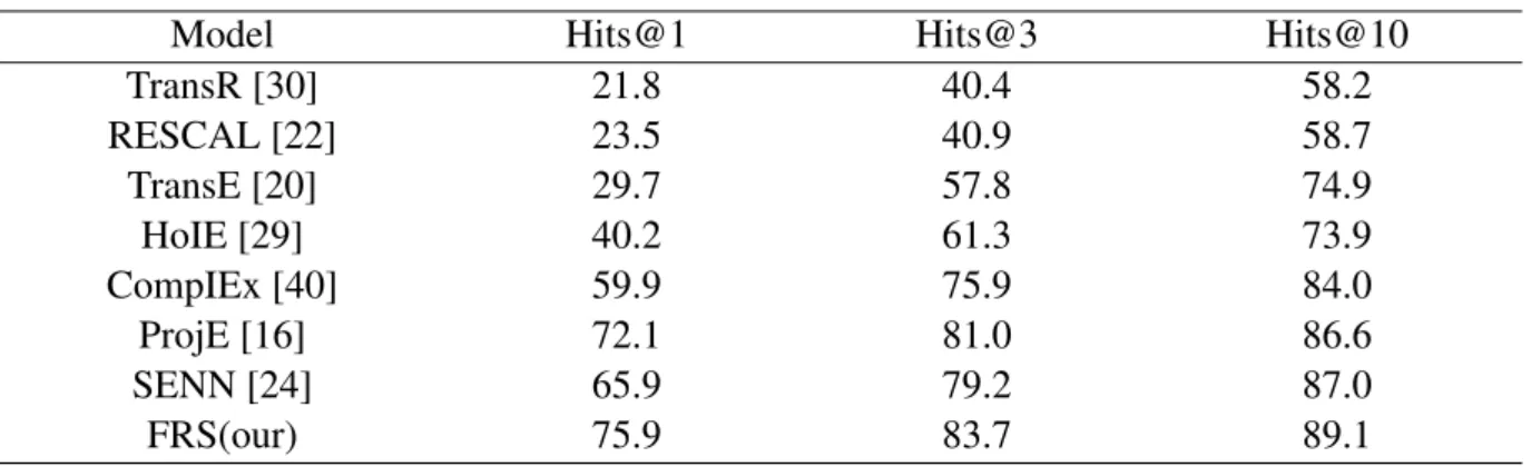
Hits@K measures if correct entities appear within the top-k elements. The higher the Hits@K, the performance of the entity prediction will be better. To better demonstrate the performance of the FRS model in terms of Hits@K, we report the experimental results compared to the representative baseline methods for fine-grained evaluation indicators in Table 6. As can be seen from Table 6, FRS
consistently outperforms all baselines in terms of three indicators, indicating that the algorithm can
further improve performance due to its effectiveness and superiority of FRS. In the comparison of
Hits@1, Hits@3, and Hits@10, they were 3.8%, 2.7% and 2.1% higher, respectively, than the best results of baseline methods.
Table 6.Experimental results of entity prediction in terms of Hits@{1,3,10}on FB15K.
Model Hits@1 Hits@3 Hits@10
TransR [30] 21.8 40.4 58.2 RESCAL [22] 23.5 40.9 58.7 TransE [20] 29.7 57.8 74.9 HoIE [29] 40.2 61.3 73.9 CompIEx [40] 59.9 75.9 84.0 ProjE [16] 72.1 81.0 86.6 SENN [24] 65.9 79.2 87.0 FRS(our) 75.9 83.7 89.1 6. Further study
For our model, there are two pivotal hyperparameters which have an influence on the evaluation
results: the embedding sizek and the probability of negative candidate sampling pn. In this section,
we focus on the impact of these two hyperparameters on the performance of the model according to the control variable method. We choose the KGE model named ProjE [16] for the analysis of
hyperparameter effects. Because FRS simply uses a specific matrix operation to combine entities and
relationships before introducing feature engineering, this is consistent with the idea in ProjE. The FB15K dataset contains more categories of relationships, it is more helpful for objective analysis of the model and the impact of parameters on the model, so the experiments in this section are designed
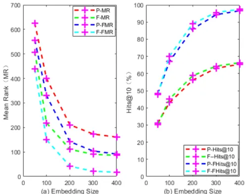
for FB15K. Figure 3 provides the effect of embedding size on FB15K. Figure 4 provides the effect of
the negative candidate sampling probability on FB15K. 6.1. The effect of embedding size
It can be seen from Figure 3(a) that both MR and FMR show a downward trend with the increase of
the embedding sizek, and the FRS decreases more than the ProjE model. It can be seen from Figure
3(b) that Hits@10 and FHits@10 both show an upward trend with the increase of the embedded sizek, and the FRS rises more than the ProjE model. Therefore, we can conclude that as the embedding size increases, the entity prediction performance of the KGE models will increase, but the Mean Rank is more sensitive to this influence factor than Hits@K. Under the same embedding size, the prediction performance of FRS model is better than ProjE. These two models have achieved a sharp change in embedding size 100,200, and 300, and the performance of prediction doesn’t improve significantly when the embedding size is more than 400. It shows that the appropriate embedding size makes the model more expressive; However, when the embedding size of the model increases to a certain threshold, the network will learn some unimportant features or even noise, which will cause negative
Figure 3. The effect of probability for negative candidate sampling. P refers to the ProjE model, and F refers to the FRS model.
6.2. The effect of probability for negative candidate sampling
As can be seen from Figure 4(a), both MR and FMR are on the rise as probability pnincreases. As
can be seen from Figure 4(b), Hits@10 and FHits@10 both show a decreasing trend as probabilitypn
increases. When the probability pnis increasing, both FRS and ProjE are negatively affected, but FRS
is less damaged than ProjE. Under the influence of negative influence, the prediction effect of FRS
model is still better than ProjE, which indicates that the model is more robust. From the experimental results in Figure 3 and Figure 4, we can conclude that the effect of the embedding size and the negative sampling probability on the entity prediction results is in reverse. Meanwhile, the influence of the embedding size on the model is greater than the negative sampling probability. This also shows that we should restore the semantic information in the embedding space as much as possible, that is, the sufficient interaction for the entities and relationships. In the experiment of further study, the prediction
effect of the FRS model was always better than ProjE, although sometimes the influence of parameters
on the experimental results was unfavorable.
7. Conclusion
In this paper, a knowledge graphs embedding model, based on the shared parameters, called FRS is proposed for entity prediction tasks. The FRS model innovatively introduces the feature engineering method into the entity prediction tasks, which alleviates the problem of insufficient interaction in the KGE models. In particular, the F network proposed in this paper realizes the alignment of entities and
Figure 4. The effect of probability for negative candidate sampling. P refers to the ProjE model, and F refers to the FRS model.
relationships in the same feature space. Experiments have shown that the FRS with the feature pro-cessing layer has absolutely good prediction performance compared with the traditional KGE model, and the prediction performance is better under the influence of the positive or negative influence of the
hyperparameter. The FRS model does not require pre-training and is a self-sufficient model of length
1, meanwhile, it obtains the best entity prediction results with a simple three-layer network. Although the FRS model uses the idea of shared parameters, there are still a large number of parameters in the training process. The future work is how to alleviate the problem of insufficient interaction while re-ducing the number of training parameters. Moreover, we will consider the temporal logic relations between components of the triples, such as the application of RNN or LSTM.
Acknowledgments
This work was supported in part by the National Natural Science Foundation of China under Grant 61373120. The work of this paper was supported by the Electronic Service Technology and Engineer-ing Lab, Northwestern Polytechnical University, through a Ph.D. Scholarship.
Conflict of interest
References
1. Knowledge graph, Available from: https://en.wikipedia.org/wiki/Knowledge_Graph.
2. M. H. Gad-Elrab, D. Stepanova, J. Urbani, et al., Exfakt: A framework for explaining facts over knowledge graphs and text, in Proceedings of the Twelfth ACM International Conference on Web
Search and Data Mining,ACM, (2019), 87–95.
3. C. W. Lee, W. Fang, C. K. Yeh, et al., Multi-label zero-shot learning with structured knowledge graphs, in Proceedings of the IEEE Conference on Computer Vision and Pattern Recognition, (2018), 1576–1585.
4. E. B. Hadley, D. K. Dickinson, K. Hirsh-Pasek, et al., Building semantic networks: The impact of
a vocabulary intervention on preschoolers depth of word knowledge,Read. Res. Quart.,54(2019),
41–61.
5. K. Bollacker, C. Evans, P. Paritosh, et al., Freebase: a collaboratively created graph database for structuring human knowledge, in Proceedings of the 2008 ACM SIGMOD international
confer-ence on Management of data,ACM, (2008), 1247–1250.
6. Wikidata, Available from:https://www.wikidata.org/wiki/Wikidata:Main_Page.
7. C. Bizer, J. Lehmann, G. Kobilarov, et al., Dbpedia-a crystallization point for the web of data, Web
Semantics: Science, Services and Agents on The World Wide Web,7(2009), 154–165.
8. T. Young, D. Hazarika, S. Poria, et al., Recent trends in deep learning based natural language
processing,IEEE Comput. Intell. M.,13(2018), 55–75.
9. B. Shi and T. Weninger, Open-world knowledge graph completion, in Thirty-Second AAAI Con-ference on Artificial Intelligence, 2018.
10. C. Meilicke, M. Fink, Y. Wang, et al., Fine-grained evaluation of rule-and embedding-based systems for knowledge graph completion, in International Semantic Web Conference, Springer, (2018), 3–20.
11. D. Q. Nguyen, An overview of embedding models of entities and relationships for knowledge base
completion,arXiv preprint arXiv:1703.08098.
12. H. Wang, F. Zhang, M. Hou, et al., Shine: Signed heterogeneous information network embedding for sentiment link prediction, in Proceedings of the Eleventh ACM International Conference on
Web Search and Data Mining,ACM, (2018), 592–600.
13. R. Xie, Z. Liu, J. Jia, et al., Representation learning of knowledge graphs with entity descriptions, in Thirtieth AAAI Conference on Artificial Intelligence, 2016.
14. Q. Wang, Z. Mao, B. Wang, et al., Knowledge graph embedding: A survey of approaches and
applications,IEEE T. Knowl. Data En.,29(2017), 2724–2743.
15. T. Zhen, Z. Xiang, F. Yang, et al., Knowledge graph representation via similarity-based
embed-ding,Sci. Programming,2018(2018), 1–12.
16. B. Shi and T. Weninger, Proje: Embedding projection for knowledge graph completion, in Thirty-First AAAI Conference on Artificial Intelligence, 2017.
17. A. Bordes, X. Glorot, J. Weston, et al., A semantic matching energy function for learning with
18. A. Bordes, J. Weston, R. Collobert, et al., Learning structured embeddings of knowledge bases, in Twenty-Fifth AAAI Conference on Artificial Intelligence, 2011.
19. T. Mikolov, I. Sutskever, K. Chen, et al., Distributed representations of words and phrases and their compositionality, in Advances in neural information processing systems, (2013), 3111–3119. 20. A. Bordes, N. Usunier, A. Garcia-Duran, et al., Translating embeddings for modeling
multi-relational data, in Advances in neural information processing systems, (2013), 2787–2795. 21. Z. Wang, J. Zhang, J. Feng, et al., Knowledge graph embedding by translating on hyperplanes, in
Twenty-Eighth AAAI conference on artificial intelligence, 2014.
22. M. Nickel, V. Tresp and H. P. Kriegel, A three-way model for collective learning on
multi-relational data., inICML,11(2011), 809–816.
23. R. Socher, D. Chen, C. D. Manning, et al., Reasoning with neural tensor networks for knowledge base completion, in Advances in neural information processing systems, (2013), 926–934.
24. S. Guan, X. Jin, Y. Wang, et al., Shared embedding based neural networks for knowledge graph completion, in Proceedings of the 27th ACM International Conference on Information and
Knowl-edge Management,ACM, (2018), 247–256.
25. Y. Lin, X. Han, R. Xie, et al., Knowledge representation learning: A quantitative review.
26. K. Xu, C. Li, Y. Tian, et al., Representation learning on graphs with jumping knowledge networks, arXiv preprint arXiv:1806.03536.
27. D. H. Pham and A. C. Le, Learning multiple layers of knowledge representation for aspect based
sentiment analysis,Data Knowl. Eng.,114(2018), 26–39.
28. K. He, X. Zhang, S. Ren, et al., Identity mappings in deep residual networks, in European confer-ence on computer vision, Springer, (2016), 630–645.
29. M. Nickel, L. Rosasco and T. Poggio, Holographic embeddings of knowledge graphs, in Thirtieth Aaai conference on artificial intelligence, 2016.
30. Y. Lin, Z. Liu, M. Sun, et al., Learning entity and relation embeddings for knowledge graph completion, in Twenty-ninth AAAI conference on artificial intelligence, 2015.
31. Z. Wang and J. Z. Li, Text-enhanced representation learning for knowledge graph., in IJCAI,
(2016), 1293–1299.
32. S. He, K. Liu, G. Ji, et al., Learning to represent knowledge graphs with gaussian embedding, in Proceedings of the 24th ACM International on Conference on Information and Knowledge
Management,ACM, (2015), 623–632.
33. G. Ji, S. He, L. Xu, et al., Knowledge graph embedding via dynamic mapping matrix, in Pro-ceedings of the 53rd Annual Meeting of the Association for Computational Linguistics and the
7th International Joint Conference on Natural Language Processing (Volume 1: Long Papers), 1
(2015), 687–696.
34. H. G. Yoon, H. J. Song, S. B. Park, et al., A translation-based knowledge graph embedding pre-serving logical property of relations, in Proceedings of the 2016 Conference of the North Amer-ican Chapter of the Association for Computational Linguistics: Human Language Technologies, (2016), 907–916.
35. H. Xiao, M. Huang, L. Meng, et al., Ssp: semantic space projection for knowledge graph embed-ding with text descriptions, in Thirty-First AAAI Conference on Artificial Intelligence, 2017. 36. G. Ji, K. Liu, S. He, et al., Knowledge graph completion with adaptive sparse transfer matrix, in
Thirtieth AAAI Conference on Artificial Intelligence, 2016.
37. H. Xiao, M. Huang and X. Zhu, Transg: A generative model for knowledge graph embedding, in Proceedings of the 54th Annual Meeting of the Association for Computational Linguistics
(Vol-ume 1: Long Papers),1(2016), 2316–2325.
38. L. Chang, M. Zhu, T. Gu, et al., Knowledge graph embedding by dynamic translation, IEEE
Access,5(2017), 20898–20907.
39. Y. Lin, Z. Liu, H. Luan, et al., Modeling relation paths for representation learning of knowledge
bases,arXiv preprint arXiv:1506.00379.
40. T. Trouillon, J. Welbl, S. Riedel, et al., Complex embeddings for simple link prediction, in Inter-national Conference on Machine Learning, (2016), 2071–2080.
c
2019 the Author(s), licensee AIMS Press. This
is an open access article distributed under the
terms of the Creative Commons Attribution License (http://creativecommons.org/licenses/by/4.0)