A Quantitative Assessment of the Decline in the U.S. Saving Rate

A Quantitative Assessment of the Decline in the U.S. Saving

Rate

Kaiji Cheny _{Ay¸se ·Imrohoro¼glu}z _{Selahattin ·Imrohoro¼glu}z

First Version October 2005; this Version January 2007

Abstract

The saving rate in the U.S. has been declining since 1960s. There have also been signi…cant secular changes in population growth, tax rates on labor and capital, and the depreciation rate of capital in this period. We use the standard growth theory calibrated to the U.S. data to evaluate the quantitative role of these factors in contributing to the decline in the saving rate. Our …ndings indicate that the decline in the population growth rate and the increase in the depreciation rate are signi…cant in explaining the secular trends, where as the medium term ‡uctuations in the total factor productivity seem important in driving the year-to-year movements in the U.S. saving rate since the 1960s.

Department of Economics, University of Oslo

z_{Department of Finance and Business Economics, Marshall School of Business,} Uni-versity of Southern California, Los Angeles, CA 90089-1427.

We would like to thank the seminar participants at USC, University of California at Riverside, Federal Reserve Bank of Chicago, Conference on Economic Dynamics at the University of Tokyo, 2006 Annual

1

Introduction

The net national saving rate in the U.S. has declined from an average of 15% in 1960s to 10% in 1980s and 8.6% in 1990s. This secular decline has occupied center stage in policy discussions and continues to attract media coverage. Understanding this decline as well as the di¤erences in saving rates across countries has also been an important part of academic research. Detailed data analyses have been conducted to explore whether particular cohorts are responsible for the low saving rate by examining personal saving rates in the U.S. For example, Gokhale, Kotliko¤, and Sabelhaus (1996) attribute the decline in the saving rate to the redistribution of resources through social security and medicare, from young consumers with low marginal propensities to consume, to older generations with high marginal propensities to consume. Attanasio (1998) argues that cohorts born between 1925 and 1939 may be to blame for the low personal saving rate. Summers and Carroll (1987) suggest that it is the reliance of the younger generations on social security that depresses saving in the U.S. Boskin and Lau (1988a,b) formulate a model based on longitudinal and cross-sectional microeconomic data together with aggregate time series and examine the importance of various factors a¤ecting aggregate consumption and saving in the U.S. Their results suggest that it is the decline in the saving of generations born after the great depression that may be responsible for the decline in the national saving rate. Summers, Carroll and Blinder (1987) examine the decline in the national saving rate and conclude that it has been due to a combination of federal de…cits and a continuation of a long term trend in private savings.1

Since 1960s there have been substantial changes in several variables in the U.S. that can have potentially important consequences for the behavior of the national saving rate. Between 1960 and 1980 the average population growth rate and the depreciation rate were 1.8% and 4.3%, respectively. By 2000 the population growth rate had declined to about 0% while the depreciation rate had increased to 5.3%.2 Each of these changes would reduce the demand for investment in the Solow growth model. While both of these changes would put a downward pressure on the saving rate, there were other changes in the economic environment, such as the decline in the capital income tax rate, that would have encouraged savings over this time period. In this paper we explore the quantitative implications of the changes

1

Another set of papers have focused on the possible relationship between the increase in stock prices and the boom in consumer spending. For example, see Parker (1999) and Juster, Lupton, Smith, and Sta¤ord (2000) who suggest that the signi…cant capital gains in corporate equities experienced since 1984 is responsible for the decline in the personal saving rate. Backus, Henriksen, Lambert, and Telmer (2005) argue that private saving rates are strongly and negatively correlated with the ratio of net worth to consumption. Also see Poterba (2000) for a survey.

in these and some other economic factors on the secular trends in the net national saving rate using standard growth theory.3 In particular, we use a one-sector, neoclassical growth model with an in…nitely-lived representative agent facing complete markets and calibrate the economy to the U.S. data for the 1960-2004 period. Our exogenous driving forces are the population growth rate, tax rates on capital and labor income, share of government expenditures in output, depreciation rate, and actual time series data for the TFP growth rate. We conduct deterministic simulations, as in Hayashi and Prescott (2002), and perform an ‘accounting exercise’to evaluate the impact of several factors that may explain the secular trends in the saving and consumption behavior.

In analyzing the saving rate, we focus our attention on the time period between 1960 and early 1990s.4 We …nd that the model generated saving rate, consumption-output ratio and the rate of return to capital resemble the data reasonably well until the 1990s. The model generated saving rate declines from an average of 17% in 1960s to about 8% by 1990. Our results suggest that the decline in the population growth rate and the increase in the depreciation rate alone account for 3-4 percentage point decline in the saving rate by early 1990s. Changes in the TFP growth rate generate annual ‡uctuations in the saving rate that resemble the data reasonably well but do not contribute to the secular decline in the saving rate. We examine the performance of the model with respect other variables, including labor supply and the rate of return to capital, and conclude that the model performance deteriorates after the 1990s.

The paper is organized as follows. Section 2 presents the growth model we use to evaluate U.S. consumption and saving behavior. Data and calibration issues are discussed in Section 3, quantitative …ndings and the sensitivity analysis are presented in Section 4. Concluding remarks are given in Section 5. Appendix A contains calibration details and data sources.

2

The Growth Model

There is a stand-in household with Nt working-age members at date t, that solves

max 1 X t=0 t_N t(logct+ log(1 ht)) 3

Our approach is in line with the recent use of the one-sector growth model to explain ‘Great Depressions’. In particular, we follow the methodology of Cole and Ohanian (1999, 2002, 2004), Kehoe and Prescott (2002), and Chen, ·Imrohoro¼glu and ·Imrohoro¼glu (2006a) in using an applied general equilibrium setup to account for the observed time path of the U.S. saving behavior.

4_{We focus on this time period for three reasons. First, our model abstracts from intangible capital and}

capital gains that seem to be relatively important after 1990s. Second, the model generated saving rate after 1990s is sensitive to our assumptions on economic factors beyond 2004. Third, our closed economy abstraction

subject to

Ct+Xt (1 h;t)wtHt+rtKt k;t(rt t)Kt+T Rt t;

where ct =Ct=Nt is per member consumption, ht= Ht=Nt is the fraction of hours worked per member of the household, is the subjective discount factor, is the share of leisure in the utility function, Htis total hours worked by all working-age members of the household, h;t and k;t are tax rates on labor and capital income, respectively, at timet; wtis the real wage,T Rtis a government transfer, tis a lump sum tax,rtis the rental rate of capital, and t is the time-tdepreciation rate. The size of the household evolves over time exogenously at the rate nt = Nt=Nt 1: Households are assumed to own the capital, Kt; and rent it to businesses.

The economy-wide resource constraint is given by

Ct+Xt+Gt=Yt;

where aggregate consumption, investment and government purchases add up to aggregate output. The law of motion for the capital stock is given by Kt+1 = (1 t)Kt+Xt:

The aggregate production function is given by

Yt=AtKt(Ht)1 ;

where is the income share of capital and At is total factor productivity, which grows exogenously at the rate gt=At=At 1.

2.1 Government

There is a government that taxes income from labor and capital (net of depreciation) and uses the proceeds to …nance exogenous streams of government purchasesGtand government transfers T Rt:A lump sum tax t is used to ensure that the government budget constraint is satis…ed each period:

Gt+T Rt= h;twHt+ k;t(rt t)Kt+ t:

In other words, t is the primary government de…cit in the model.

2.2 Competitive Equilibrium

Given a government policy _fGt; T Rt; h;t; k;t; tg1t=0, a competitive equilibrium consists of

an allocation _fCt; Xt; Ht; Kt+1; Ytg1t=0 and price systemfwt; rtg such that given policy and prices, the allocation solves the household’s problem,

given policy and prices, the allocation solves the …rm’s pro…t maximization problem with factor prices given by: wt= (1 )AtKt(Ht) ;and rt= AtKt 1(Ht)1 ; the government budget is satis…ed,

and the goods market clears: Ct+Xt+Gt=Yt:

2.3 Numerical Solution

Our numerical solution procedure follows Hayashi and Prescott (2002). After calibrating the model parameters and exogenous variables, we …rst compute a steady-state assumed for the U.S. economy in a su¢ ciently distant future. To obtain this steady-state, we write down the equilibrium conditions of the model, detrend variables to induce stationarity, and then impose these steady-state conditions. Once the steady-state is obtained, we use a shooting algorithm toward this …nal steady state from given initial conditions in 1960. This solution method yields an equilibrium transition path from initial conditions toward a steady-state.

Equilibrium Conditions: The equilibrium conditions of this model can be described

in three equations below:

ht 1 ht = (1 h;t)(1 ) Yt Ct ; (1) Ct+1 Nt+1 = Ct Nt n 1 + (1 k;t+1) h At+1K_t+11(Ht+1)1 t+1 io ; (2) Kt+1 = (1 t)Kt+AtKt(Ht)1 Ct Gt: (3)

Detrending: For an aggregate variable zt; its detrended version is given by: ezt =

zt= A 1 1

t Nt :Applying this change of variables to (2) and (3), we obtain equations

e ct+1 = e ct g 1 1 t+1 n 1 + (1 k;t+1) h x_t+11 t+1 io ; e kt+1 = 1 g 1 1 t+1nt+1 [(1 t) + (1 t)xt 1]ekt ect;

where _t is the ratio of government purchases to output,Gt=Yt;andxt is detrended capital-labor ratio,(Kt=Ht)=A

1 1

t :

Steady-state: Setting z_et = ze for all t; we obtain the following steady-state for the

model: e h 1 eh = (1 eh)(1 ) e y ec 1 = 1 g11 n 1 + (1 _ek) h x 1 eio

These equations are solved for the steady-state values of detrended capital, consumption and hours worked where e; _eh; and ek are the steady-state depreciation, labor income tax rate and capital income tax rate, respectively. The steady-state saving rate is given by

e s= (g 1 1 _{n 1)}e_k e y eek : (4)

Transition to the steady-state: Starting from a given value of the initial capital

stock K0; we guess a value for the endogenous variable C0 and use equations (1) to(3) to

obtain a path for the endogenous variablesCt,HtandKt+1 towards the steady-state. If this

path is not achieved, we iterate on the initial guess for C0 using this ‘shooting’ algorithm

until convergence to the steady-state is obtained. Equipped with the equilibrium path ofCt; Ht and Kt+1; we can then use other equilibrium conditions to construct time paths of all

aggregate quantities and prices. In particular, we compute the saving rate using5

st=

Yt Gt Ct tKt Yt tKt

:

3

Calibration

We calibrate the model economy using data from the 2005 revision of National Income and Product Accounts (NIPA), Fixed Asset Tables (FAT) of Bureau of Economic Analysis (BEA), Statistics of Income (SOI), Individual Income Tax Returns (1960-2003), and the Social Security Bulletin.

Constant Parameters: There are 3 parameters that are time invariant throughout our

analysis. The capital share parameter, ; is set to its average value of0:4 over our sample period 1960-2004. The subjective discount factor, ; is set to 0:9702 so that the capital output ratio is 3:2 at the …nal steady state. The share of leisure in the utility function, ;

is set to 1:45 to match an average workweek of 35 hours. These choices are summarized below.

Time-Invariant Parameters

0:4 1960-2004 average

0:9702 Target: K=Y = 3:2in steady state

1:45 Target: Average workweek = 35hours

5

We treat the model as a closed economy where net national saving and investment are identical. This abstraction is better suited up to 1990s. A two-country model for the later time periods would be useful especially if the aim is to understand the current account de…cits. However, since we are interested in understanding the secular decline in the saving rate, the closed economy assumption seems su¢ cient. See for example, Henriksen (2006) and Krueger and Ludwig (2006) who construct open economy models and analyze

Calibration of the Steady-State (2070 and Beyond) and 2005-2070: We assume that the U.S. economy starts from given conditions in 1960 and eventually converges to a steady-state in 2070.6 In order to characterize this steady-state equilibrium, we use the following values for model variables, starting from year 2005:

Steady-State Values: 2005 and Beyond

gt 1 TFP Growth Rate 0.0142

nt 1 Population Growth Rate 0.01

t Government Purchases to GNP Ratio 0.14

t Depreciation Rate 0.05

T Rt=GN P Transfers to GNP Ratio 0.10

k;t Capital Income Tax Rate 0.40

h;t Labor Income Tax Rate 0.276

In our benchmark model, we set the seven exogenous variables in the above list equal to their long-run averages.7 Note that the population growth rate in the U.S. has been declining since the 1960s and according to the Census Bureau projections it will continue at very low rates in the future. Thus, we set the population growth rate after 2004 and at the steady state equal to 1% which is smaller than the average population growth rate of1:5%

between 1960-2004.8 Similarly, the depreciation rate has been increasing in the U.S. For the periods after 2004 and at the steady state, we set the depreciation rate equal to 5%which is the average depreciation rate between 1990-2004.9 We discuss the sensitivity of our results to the assumptions made for the periods beyond 2004 in the section on sensitivity analysis.

Calibration of the 1960-2004 period: In our benchmark simulation, we use the actual

time series data between 1960-2004 for the following exogenous variables: TFP growth rate,

gt 1; population growth rate, gt 1; depreciation rate, share of government purchases in GNP, _t;share of government transfers in GNP,T Rt=GN Pt;and capital and labor income tax rates, k;t; h;t.10 Empirical marginal tax rates are constructed using the methods of

6_{This is an approximation. Allowing for a longer transition period from 1960 for convergence to a}

steady-state has no quantitative impact on the 1960-2004 period we are investigating.

7_{With our assumed tax rates, the government budget will be in a surplus at the steady state.}

8_{Population growth rates are the growth rates of civilian non-institutional population 16 years and over}

reported by the BLS.

9

Gomme and Rupert (2005) provide detailed calculations for the depreciation rate of di¤erent types of capital. Increasing depreciation rates are evident in computers and to some extent in market structures since 1960s.

Joines (1981) and McGrattan (1994). The data used in the calibration are provided in the Appendix. We compute the initial capital-output ratio in 1960 as 3:5 and take it as a given initial condition.

4

Results

We start this section by presenting several deterministic simulations and counterfactual ex-periments to assess the impact of various exogenous variables on the saving rate. We later examine the sensitivity of our results to some of the key assumptions present in the bench-mark calibration and run two experiments with stochastic TFP growth rates. In all the experiments, we graph simulated saving rates between 1960 and 2004. However, in analyz-ing the secular trend in the savanalyz-ing rate we focus our attention to the time period between 1960 and early 1990s for three reasons. First, as we later show the model generated saving rate after 1990s is sensitive to our assumptions on economic factors, especially the TFP growth rate, beyond 2004. In addition, our model abstracts from intangible capital and capital gains that seem to be relatively important after 1990s. Also, our closed economy abstraction is better suited up to the 1990s.

4.1 Main Findings

In Figure 1 we display the actual net national saving rate as well as the model generated saving rate for the benchmark calibration. The model does reasonably well in terms of capturing most of the secular decline between 1960 and early 1990s, as well as the annual ‡uctuations, in the actual U.S. data. For example, the model generated saving rate declines from an average of 17% in 1960s to about 8% by 1990. Net national saving rate in the U.S. has declined from an average of 15% in 1960s to 8.6% in 1990s. However, the model generated saving rate is considerably larger than the data in the mid 1960s and smaller than the data between 1975 and 1990.

where the capital share is set to 0:4, Yt is GN P plus service ‡ow from the stock of consumer durables and government capital, Kt is capital stock inclusive of foreign capital, stock of consumer durables and government capital, and Ht is aggregate hours worked. In this framework investment consists of domestic private investment and the current account surplus. Even though we treat the model as a closed economy, we include the foreign capital in the de…nition of the capital stock to make sure that the TFP growth rates faced by the U.S. individuals can be accurately measured. However, it is important to note that this adjustment is quantitatively very small. None of the results are signi…cantly altered by di¤erent measurements of TFP such as inclusion of government capital or the exclusion of foreign capital. Gomme and Rupert (2005) provide three di¤erent measures of the U.S. TFP growth rate based on very di¤erent assumptions on the capital stock. The TFP growth rates implied by their results as well as ours display very similar properties over this time period.

0.00 0.05 0.10 0.15 0.20 0.25 1960 1965 1970 1975 1980 1985 1990 1995 2000 Saving Rate Data Model

Figure 1: Data and the Model

In order to understand the main factors behind the behavior of saving over this time period, we conduct several counterfactual experiments. In our benchmark economy, we have used time series data for the TFP growth rate, population growth rate, depreciation rate, capital and labor income tax rates, and fraction of government expenditures in GNP. During 1960-2004 there was a signi…cant decline in the population growth rate and an increase in the depreciation rate that are displayed in …gures A2 and A3 in the Appendix. In addition, there was a decrease in the capital income tax rate and an increase in the labor income tax rate. To isolate the impact of these changes one at a time, we start with setting all the exogenous variables equal to their sample averages. Later we add the time series data for each exogenous variable one at a time.

Population Time Series Only: In our …rst counterfactual experiment we try to isolate

the role of the declining population growth rate by simulating the saving rate in an economy where all the exogenous variables (TFP growth, G/Y, depreciation, tax rates, transfers) are set to their long-run averages except for the population growth rate. In Figure 2, the series labeled ‘Population Time Series Only’ displays the saving rate that is generated by the model economy where the only time series data that is used in the simulations is the population growth rate. The quantitative impact of the population growth rate in this time period seems moderate, resulting in a 1-2% decline by early 1990s.

0.04 0.06 0.08 0.10 0.12 0.14 0.16 0.18 1960 1965 1970 1975 1980 1985 1990 1995 2000 Saving Rate Data

Population Time Series Only

Figure 2: Role of Population Growth

Declining Population Growth Rate and Increasing Depreciation Rate: In

Fig-ure 3 we conduct an experiment that quanti…es the role of the population growth rate together with the depreciation rate. The depreciation series we construct from adjusted NIPA data indicates a slight increase over time which alone would result in a decrease in the saving rate. The series labeled ‘Time Series for Population and Depreciation’ displays the simulated saving rate from this experiment. The increase in the depreciation rate and the decrease in the population growth rate together account for 3-4 percentage point decline in the saving rate by early 1990s.

0.04 0.06 0.08 0.10 0.12 0.14 0.16 0.18 1960 1965 1970 1975 1980 1985 1990 1995 2000 Saving Rate

Time Series for Population and Depreciation Data

Figure 3: Role of the Population Growth and Depreciation

All Time-Varying Except TFP Growth Rate: In Figure 4 we generate the saving

rate in an economy where time series values of all the exogenous variable except the TFP growth rate are used in the simulations. Thus in this environment, tax rates, government expenditures, population growth rate and the depreciation rate all take their time series values whereas the TFP growth rate is set to its long-run average. Notice that the resulting saving rate is able to capture some of the secular decline in the saving rate. However, the simulated saving rate does not generate the decline observed in the data in late 1980s and late 1990s.

0.04 0.06 0.08 0.10 0.12 0.14 0.16 0.18 1960 1965 1970 1975 1980 1985 1990 1995 2000 Saving Rate Data All except TPF growth rate

are equal to their time series values

Figure 4: All Except TFP

TFP Growth Rate Only: Next, we examine the model generated saving rate when the

only time series data that is included in the simulations is the TFP growth rate. We set all the other exogenous variables equal to their long-run averages. There are several interesting features of the model generated saving rate that is displayed in Figure 5. First, it displays signi…cant ‡uctuations that mimic the data rather well until 1975. There is a sharp decline in the model generated saving rate in the early 1980s and late 1990s, and a sharp increase in the early 1990s.

0.00 0.02 0.04 0.06 0.08 0.10 0.12 0.14 0.16 0.18 0.20 1960 1965 1970 1975 1980 1985 1990 1995 2000 Saving Rate Data

TFP Time Series Only

Figure 5: Role of TFP

To understand the relationship between TFP growth and the saving behavior better, we display these two series in Figure 6. Since we are conducting deterministic simulations, households know the entire path of the TFP growth rate and make decisions on how much to save based on this information. In general, periods with high TFP growth are associated with high return to capital and high saving rates. For example, the model generates a relatively high saving rate between 1990-1995 which is a period of relatively high TFP growth. The decline in the TFP growth rate in 2001 results in a sharp decline in the saving rate.

0 0.02 0.04 0.06 0.08 0.1 0.12 0.14 0.16 0.18 0.2 1961 1966 1971 1976 1981 1986 1991 1996 2001 Saving Rate 0.920 0.940 0.960 0.980 1.000 1.020 1.040 1.060 TFP growth rate

Model Saving Rate

TFP Growth Rate

Figure 6: TFP Growth and the Saving Rate

Overall, our results suggest that i) the decline in the population growth rate and the increase in the depreciation rate alone account for 3-4 percentage point decline in the saving rate, ii) observed TFP growth rates alone would have caused the saving rate to be much higher in the 1990-1995 period, and, iii) the decline in the TFP growth rate in 2001 had a signi…cant negative impact on the saving rate.

4.2 Additional Properties and Sensitivity Analysis

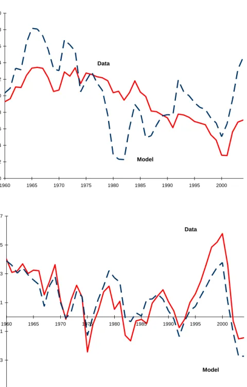
Labor Input, Return to Capital, and Consumption: In this section we examine

additional properties of the benchmark economy by comparing the simulated series for labor, capital, interest rate, and consumption output ratio with their counterparts in the data. Our results indicate that the model economy works reasonably well in mimicking some aspects of the data but not all. In Figure 7 we display the observed time series path of the labor input and the after-tax return to capital (calculated from NIPA) and compare them with those generated by our model. In the …rst panel, we display data for total hours per capita.11 Notice that the model generated series displays a decline in the labor input while the total hours in the data do not decline. In our simple model, the decrease in simulated hours is mainly driven by the fact that tax rates on labor increase steadily over the past forty years.

Therefore, with perfect anticipation of this trend, the stand-in household tends to substitute hours in the early periods for hours in the late periods. McGrattan and Rogerson (2004) show that the increase in hours per capita observed in the U.S. is mainly due to the increase in the labor force participation rate of females. In fact, employment to population ratio of women increases by 87% in this time period while that of men declines by 15.7%. The simple framework used in this model is not capable of mimicking these trends.12 In order to document the sensitivity of the simulated saving rate on this feature of the model we generate the saving rate taking the labor input exogenously from the data. We …nd that the secular decline in the saving rate generated in this model is very similar to our results from the benchmark model with endogenous labor until 1990s. After this period, the model with exogenous labor generates higher saving rates than our benchmark model.

In the second panel, we display the after-tax rate of return to capital in the data and the model economy. Although the …t from 1960 to early 1990s seems reasonably good, there is a major discrepancy between the two series in the late 1990s. One potential reason for this discrepancy may be the increase in the capital’s share in total income in 1990s as documented by, for example, Gomme and Rupert (2005). This share is constant in our Cobb-Douglas production speci…cation.13 Part of the large increase in the rate of return to capital in the data is also due to the increase in corporate pro…ts that incorporate the large increase in capital gains in the 1990s. Our one sector growth model abstracts from such valuation e¤ects.

The third panel of the graph displays the consumption output ratio in the data against the simulated series. Although the secular movements seem to be reasonably characterized, the model has di¢ culty mimicking the observed behavior in certain subperiods.

1 2

Several papers investigate the rise of the female labor force participation such as Jones, Manuelli and McGrattan (2003), Olivetti (2001), Akbulut (2005), and Caucutt, Guner, and Knowles (2002).

1 3_{Notice that the after-tax rate of return for capital in the data is positively correlated with capital share}

in total income and negatively correlated with the capital-output ratio, while in our model it is driven by capital-output ratio alone. Therefore, to the extent that capital’s share in total income has increased during the 1990s, our model would underestimate the increase in the after-tax return to capital.

0.10 0.15 0.20 0.25 0.30 0.35 0.40 0.45 1960 1965 1970 1975 1980 1985 1990 1995 2000 Labor Model Hours per capita- Data

0.010 0.020 0.030 0.040 0.050 0.060 0.070 1960 1965 1970 1975 1980 1985 1990 1995 2000

After Tax Net Return

to Capital Model Data 0.52 0.54 0.56 0.58 0.60 0.62 0.64 0.66 0.68 C/Y Data Model 15

Private and Public Saving Rates: It is also possible to separate the net national saving rate in this economy into its two components and examine the private and the gov-ernment saving rates separately. In Figure 8 we display the simulated series against their counterparts in the data. Notice that while the simulations take the tax rates and the government consumption directly from the data, there is no guarantee that the simulated government saving rates should mimic the data well. To the extent that the model gener-ated labor and capital series are similar to their counterparts in the data, the government revenues generated by the model will capture the data. As can be seen from the second panel of Figure 9, the simulated government saving rates look reasonably close to data.14 The private saving rate captures all the discrepancies that were present in the earlier results for the net national saving rate. The model generated saving rates are very low after 1975 and very high in 2004.

1 4_{It is important to note that we have to make an adjustment to our de…nition of the capital stock,}

which includes the stock of durable goods and government capital, when we are calculating the tax revenues generated from capital income. In the NIPA data, these two components are not taxed at the capital income tax rate. Thus we take them out of the de…nition of capital when we are computing the tax revenues from capital income.

0.00 0.02 0.04 0.06 0.08 0.10 0.12 0.14 0.16 0.18 0.20 1960 1965 1970 1975 1980 1985 1990 1995 2000

Private Saving Rate

Data Model -0.05 -0.03 -0.01 0.01 0.03 0.05 0.07 1960 1965 1970 1975 1980 1985 1990 1995 2000 Gover nment Saving Rate Data Model

Figure 8: Private and Government Saving

Alternative Assumption on Values for 2005 and Beyond: Our procedure for

assigning values to TFP growth rates between 2005 and the …nal steady-state is arbitrary. In our benchmark calculations we set the TFP growth rate equal to its 1960-2004 average right after 2004. To check the sensitivity of our results to this assumption, we report simulations

higher than its steady state value. In Figure 9, the vertical line represents the year 2004 beyond which the two simulated saving rates di¤er only because of the assumed values for the TFP growth rate for 2005 and beyond. There are noticeable di¤erence in the 1990-2004 period between the two series. However, the two series are virtually identical until the 1990s which is one of the reasons why focus our results up to the 1990s.15

1 5

Among the exogenous variables for which we had to make assumptions about future values, TFP growth rate was the most imporant. The rest of the variables had insigni…cant consequences in the results up to 2004.

0.00 0.05 0.10 0.15 0.20 0.25 1960 1970 1980 1990 2000 2010 Saving Rate High future TFP Low future TFP Data 0.50 0.52 0.54 0.56 0.58 0.60 0.62 0.64 0.66 0.68 1960 1970 1980 1990 2000 2010 C/Y High future TFP Low future TFP

Figure 9: Role of the Future

4.3 No Perfect Foresight

assumptions on expectations for the TFP growth rate while we still feed in the time path of all the other exogenous variables deterministically.

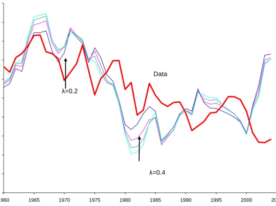
Adaptive Expectations: Our …rst alternative expectations scheme is a simple adaptive

framework where expectations of future TFP growth rates are formed according to

ge_t+1 =g_te+ (gt gte):

Here, the parameter ₂ [0;1] re‡ects the extent to which expectations will change as a result of past errors. A near zero indicates near-static expectations whereas a near unity suggests setting expectations equal to the most recently observed actual growth rate. In the latter case, the model’s saving rate would essentially shift one period hence relative to our perfect foresight case.

0 0.02 0.04 0.06 0.08 0.1 0.12 0.14 0.16 0.18 0.2 1960 1965 1970 1975 1980 1985 1990 1995 2000 2005 Saving Rate λ=0.2 λ=0.4 Data

Figure 10: Saving Rate with Adaptive Expectations

Figure 10 displays observed saving rates and a collection of simulated saving rates indexed by a few values of : Even the near-static expectations cases with low values of generate saving rates with similar features compared to the deterministic case. The secular movements are reasonably well-represented, but the model does a poor job in the 1980s and early 2000s.

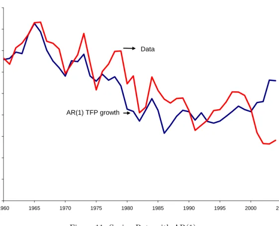
Stochastic TFP Growth Rate: Another alternative formulation is to assume that

per-sistence coe¢ cient of 0.33 (with an intercept term 0.69 and a standard error of regression 0.0224). 0 0.02 0.04 0.06 0.08 0.1 0.12 0.14 0.16 0.18 1960 1965 1970 1975 1980 1985 1990 1995 2000 2005 Saving R ate Data AR(1) TFP growth

Figure 11: Saving Rate with AR(1)

Figure 11 depicts the actual saving rate and the model generated saving rate when households forecast future TFP growth rates using the estimatedAR(1)process given above. The simulated saving rate is fairly close to the actual saving rate. The AR1 assumption for the TFP growth rate produces smoother saving rates compared to the perfect foresight case. Households’intertemporal behavior is subdued due to the lack of perfect foresight of the real return to capital.

5

Concluding Remarks

Why has the U.S. net national saving rate fallen from about 15 percent in 1960s to about 8.6 percent in early 1990s? A popular answer has been the decline in the private saving of We assume that agents have perfect foresight for all other exogenous variables by specifying a degenerate transition matrix with forty-six states. In this matrix, each state refers to a vector of exogenous series corresponding to a particular year and the transition probabilities from year j to j+ 1 (j 2004) is one. We set the vector of exogenous series corresponding to year 2005 as the steady state vector speci…ed in the calibration section. Also, we set the last diagonal of this matrix to one which indicates that after 2005 the

the baby boom generation in response to an increase in the generosity of the social security program. In this paper, we abstract from life cycle features and social security, and employ a standard growth model calibrated to the U.S. economy. Our in…nite horizon, complete markets setup captures the decline in the U.S. saving rate reasonably well. The important factors responsible for the secular decline between 1960 and early 1990s are i) the decrease in the population growth rate, and ii) the increase in the depreciation rate. The time path of observed TFP growth rates does not exhibit a trend but help explain the year-to-year ‡uctuations in the saving rate over this time period. Although the standard model performs well overall, the results for the periods after early 1990 are sensitive to the assumptions made about the future. The model also abstracts from several features on the U.S. economy that seem to be important especially since the 1990s. For example, Corrado, Hulten, and Sichel (2006) and McGrattan and Prescott (2006) document the importance of intangible capital since 1990s that is absent in our calculations. In addition, the model we have used can not account for the large increase in household wealth and its possible impact on the saving consumption decision. These issues together with a more detailed study of the 1990s, and the implications of a life-cycle model as in Chen, ·Imrohoro¼glu and ·Imrohoro¼glu (2006b) are left for future research.

6

Appendix

6.1 Calibration of the Benchmark Economy

In this section, we provide the details of our calibration for the benchmark economy. We use data from the 2005 revision of National Income and Product Accounts (NIPA) and Fixed Asset Tables (FAT) of Bureau of Economic Analysis (BEA) for the years 1960-2004. Our adjustments to measured macroeconomic aggregates follow Cooley and Prescott (1995).

Denote measured GNP as follows

(cs+cnd+icd) +g+i+nx+nf p=GN P =dep+N N P (A-1)

wherecs; cnd; icddenote service ‡ow of consumer durables, consumption of nondurable and expenditure on consumer durable. g denotes the sum of government consumption, denoted as gc; and gross government investment, denoted as gi. i denotes gross private investment.

nx denotes net export and nf pdenotes net factor payments on foreign assets. dep denotes consumption of …xed capital.

First, we include government capital in the de…nition of the capital stock. Once we include the service ‡ow from government capital,sg, A-1 becomes

Second, we treat the stock of consumer durable as part of capital stock. Then A-2 becomes

(cs+cnd+csd+sg) +gc+ (i+nicd+dcd+gi) (A-3)

+nx+nf p = GN P +sg+csd

= (dep+dcd) + (N N P +sg+csd dcd)

where csd is service ‡ow from consumer durable and dcd denote depreciation of consumer durable. Therefore, total private consumption becomes (cs+cnd+csd+sg) and total investment investment becomes(i+icd+gi)or(i+nicd+dcd+gi), wherenicdis referred to as net investment in consumer durable anddcddenotes depreciation of consumer durable:

Total depreciation becomes(dep+dcd):

Third, we treat net foreign asset as part of capital stock. A-3 then becomes

(cs+cnd+csd+sg) +gc (5)

+(i+nicd+dcd+gi+nx+nf p) = GN P +sg+csd (6)

= (dep+dcd) + (N N P +csd+sg dcd)

Now total investment becomes (i+nicd+dcd+gi+nx+nf p):

In summary, we de…ne capital K as the sum of the …xed assets, stock of consumer durables, inventory stock land, and net foreign assets. Output Y corresponds to GN P +

sg+csd and total depreciation corresponds to dep+dcd.

Following McGrattan and Prescott (2000), we assume that the rate of returns for con-sumer durable and government …xed assets are equal to the rate of return for non-corporate capital stock. Speci…cally, we have

i = (Accounting Returns + Imputed Returns)

(Non-corporate capital +land+inventory+Capital of Foreign Subsidiary)

= (0:0603 + 1:6803i) (2:976 + 0:0095=i)

where 0.0603 is non-corporate pro…t plus net interest less intermediate …nancial services, 1.6803 is the sum of the net stock of government capital, consumer durable, land and inven-tory; 2.976 is the sum of net stock of non-corporate business, government capital, consumer durable, land and inventory. 0.0095 is the net pro…t from foreign subsidiaries.

The above equation gives a value ofiat 3.93% over the period between 1960 and 2000.

Ysd and Ysg denote the service ‡ows from consumer durables and government capital, respectively, which are computed following Cooley and Prescott (1995).

Then the capital share in the output function is computed as

= Ykp+Ysd+Ysg

GN P +Ysd+Ysg ;

where Ykp is the income from private …xed assets

Ykp = Unambiguous capital income+ p (proprietors’income (A-5)

+indirect business tax)+depreciation (7)

= p GN P

This gives a value 0:32 for p and a value of0:41 for : De…ne the net national saving rate as

s = Y CON GOV DEP R

Y DEP R

= (GN P +sg+csd) (cs+cnd+csd+sg) gc (dep+dcd) (GN P +sg+csd) (dep+dcd)

= GN P cs cnd gc (dep+dcd)

N N P +csd+sg dcd

Since in our model government does not issue debt or lend to households, we de…ne the primary government saving rate as

sgov= Tax revenue (gc+tr) net interest payment on government liability

Y DEP R

where tr is the net government transfer, computed as current transfer payment minus current transfer receipts. Accordingly, the private saving rate is computed as

psav =s sgov

TFP level is computed as

A= Y

K (H)1

Table A1. Model Economy Account

Model Expression 1 Depreciation K 2 Labor income wH 3 Capital income rK 4 Total Income Y 5 Private Consumption C 6 Government Consumption G

Table A2. National Accounts, Average 1960-2003 Relative to GNP

Consumption of …xed capital 0.115

Compensation of employees 0.571

Unambiguous capital income17 0.154

Proprietors’Income with IVA and CCadj 0.074

Indirect Business Taxes18 0.086

Gross national income 1.000

Personal consumption expenditures 0.635

Durable goods 0.082

Nondurable goods and services 0.553

Gross private domestic investment 0.161

Government consumption expenditures and gross investment 0.206

Consumption expenditures 0.167

Gross investment 0.039

Net foreign investment19 _-0.002

Gross national product 1.000

Addendum

Consumption of …xed capital, durable goods 0.062

Consumption of government …xed assets 0.024

Net stock of government …xed assets 0.671

Net stock of consumer durable goods 0.301

1 7_{Unambiguous capital income=Rental Income of persons with CCAdj+Corporate Pro…ts with IVA and}

CCadj+Net Interest and miscellaneous payments.

1 8

Indirect business taxes are equal to the sum of tax on production and imports less subsidies, business transfer, current surplus of government enterprises and statistical discrepancy.

1 9

Table A3. Mapping From National Accounts to Model Accounts (Excluding Gov’t Capital)

Model NIPA

1 Depreciation ( K) 0.153

Consumption of …xed capital 0.115

Consumption of …xed capital, durable goods 0.062

Less: Consumption of government …xed assets -0.024

0.153

2 Labor income (wE) 0.683

Compensation of employees 0.571

0:7 (Proprietors’income +Indirect business taxes) 0.112

0.683

3 Capital income (rK) 0.228

Unambiguous capital income 0.154

0:3 (Proprietors’income +Indirect business taxes) 0.048

Imputed capital services from durable goods 0.026

0.228

4 Total income (Y) 1.064 1.064

Table A3. Mapping From National Accounts to Model Accounts (Excluding Gov’t Capital)

5 Private consumption(C) 0.641

Personal consumption expenditure 0.635

Less: Consumption expenditure, durable goods -0.082

Imputed capital ser. from durable goods20 0.026

Consumption of …xed capital, durable goods 0.062

0.641

6 Public consumption (G) 0.182

Government consumption exp. and gross investment 0.206

Less: Consumption of …xed capital, gov. capital -0.024

0.182

7 Investment (I) 0.241

Gross domestic private investment 0.161

Personal consumption expenditure, durable goods 0.082

Net foreign investment -0.002

0.241

8 Total Product (Y) 1.064 1.064

Table A4. Mapping From National Accounts to Model Accounts (Including gov’t capital)

Model NIPA

1 Depreciation ( K) 0.177

Consumption of …xed capital 0.115

Consumption of …xed capital, durable goods 0.062

0.177

2 Labor income (wH) 0.683

Compensation of employees 0.571

0:7 (Proprietors’income+Indirect business taxes) 0.112

0.683

3 Capital income (rK) 0.286

Unambiguous capital income 0.154

0:3 (Proprietors’income+Indirect business taxes) 0.048

Imputed capital services from durable goods 0.026

Imputed services from government …xed assets 0.058

0.286

4 Total income (Y) 1.146 1.146

Table A4 Mapping From National Accounts to Model Accounts (Including gov’t capital)

5 Private consumption (C) 0.699

Personal consumption expenditure 0.635

Less: Consumption expenditure, durable goods -0.082

Imputed capital services from durable goods 0.026

Imputed services from government capital21 0.058

Consumption of …xed capital, durable goods 0.062

0.699

6 Public consumption (G) 0.167

Government consumption expenditure 0.167

7 Investment (I) 0.280

Gross domestic private investment 0.161

Personal consumption expenditure, durable goods 0.082

Net foreign investment -0.002

Gross government investment 0.039

0.280

In Figure A1 we compare the data on the net national saving rate as a percent of NNP from the NIPAs with the one that results after all the adjustments discussed above are made to the data. 0.000 0.020 0.040 0.060 0.080 0.100 0.120 0.140 0.160 0.180 1960 1965 1970 1975 1980 1985 1990 1995 2000

Net National Saving - NIPA

Net National Saving -Adjusted

Figure A1: NIPA and the Adjusted Saving Rate

6.2 Computation of capital and labor income tax rates

This section brie‡y describes how we estimate the tax rates used in this paper. We use data from Statistics of Income (SOI), Individual Income Tax Returns (1960-2003), Social Security Bulletin and National Incomes and Product Accounts (1960-2003). The series of tax rates are constructed using the method of Joines (1981) and McGrattan (1994). The main di¤erence between our approach and McGrattan (1994) is that we assume 32 percent of the proprietor’s income is attributable to capital income and the remaining is attributable to labor income. This is consistent with our assumption in measuring the income of private …xed asset, Ykp. In contrast, McGrattan (1994) assumes all proprietor’s income belongs to labor income. As a result, our measurement of capital income tax rate is lower than its counterpart in McGrattan (1994). In addition, we exclude net capital gain from income subject to the personal income tax.

6.3 Computation of After-Tax Rate of Return to Capital We compute real after-tax capital income as

YKAT = YKBT realcapital income taxes where

YKBT = (net interest+corporate pro…ts+rental income

+.32 proprietor’s income+state ibt property taxes) A A = 1 + (total ibt tax state ibt property tax)=national income:

Capital income tax is computed as proportional tax on capital income, denoted asT KP;

plus the computed nonproportional tax on capital income and the proportional tax on both capital and labor income, denoted as T KN. Speci…cally

T KP = federal pro…t tax+state pro…t tax

+state property tax+state ibt property tax

and T KN is the product ofYKBT and the sum of proportional tax rate on both capital and labor income and the computed tax rate on capital income that is part of the individual income.

Finally, real after tax return to capital is computed as

RAT =

YKAT

K stock of consumer durable and government capital

where the measurement ofKis the same as that in calibration of the benchmark economy.

6.4 Data

In Figure A2 we display the growth rate of the total resident population in the U.S. between 1960 and 2015. This data is obtained from the U.S. Bureau of the Census which has projec-tions until 2099. The horizontal line in Figure A2 displays the average population growth rate in the 1960-2004 period. This value is used in the counter factual experiments where exogenous variables are set to their long-run averages.

1.000 1.005 1.010 1.015 1.020 1.025 1.030 1.035 1960 1970 1980 1990 2000 2010 Populat ion Growt h Long-run average

Figure A2: Population Growth Rate

Similarly, in Figure A3, we display the data for the depreciation rate, capital income tax rate, and labor income tax rate for the 1960-2015 period, as well as their average values for the counterfactual experiments. Notice that in the benchmark results we have assumed the values of these variables after 2004 to stay at their 2004 levels. .

0.020 0.025 0.030 0.035 0.040 0.045 0.050 0.055 0.060 1960 1970 1980 1990 2000 2010 Deprecia

tion Rate Long-run average

Benchmark values 0.02 0.07 0.12 0.17 0.22 0.27 0.32 0.37 0.42 0.47 0.52 1960 1970 1980 1990 2000 2010 Tax Rates Benchmark Capital Income Tax Rate

Benchmark Labor Income Tax

References

[1] Akbulut, R. (2005). “Topics in Women’s Labor Force Participation”. Dissertation USC Economics.

[2] Attanasio, O. (1998). “A Cohort Analysis of Saving Behavior by U.S. Households”. Journal of Human Resources, Vol 33, No3, Summer 1998, pp575-609.

[3] Backus, D., E. Henriksen, F. Lambert, and C. Telmer (2005). “Current Account Fact and Fiction”. Working paper NYU.

[4] Boskin, M., and L. Lau (1998a). “An Analysis of Postwar U. S. Consumption and Saving: Part I, The Model and Aggregation”. Working Paper No. 2605, National Bureau of Economic Research, Inc.

[5] Boskin, M., and L. Lau (1998b). “An Analysis of Postwar U. S. Consumption and Saving: Part II, Empirical Results”. Working Paper No. 2606, National Bureau of Economic Research, Inc., Cambridge, MA, June 1988

[6] Caucutt, E, N. Guner, and J. Knowles. (2002), “Why Do Women Wait? Matching Wage Inequality, and the Incentives for Fertility Delay”. Review of Economic Dynamics, Vol. 5, No. 4, October, pp. 815— 55.

[7] Chen, K., A. ·Imrohoro¼glu and S. ·Imrohoro¼glu (2006a). “The Japanese Saving Rate”. Forthcoming in American Economic Review.

[8] Chen, K., A. ·Imrohoro¼glu and S. ·Imrohoro¼glu (2006b). “The Japanese Saving Rate between 1960-2000: Productivity, Policy Changes, and Demographics”. Forthcoming Economic Theory.

[9] Cole, H. L. and L. E. Ohanian (1999). “The Great Depression in the United States from a Neoclassical Perspective”. Federal Reserve Bank of Minneapolis Quarterly Review, 23, 2-24.

[10] Cole, H. and L. Ohanian (2002). “The Great U.K. Depression: A Puzzle and Possible Resolution”. Review of Economic Dynamics, Vol. 5, No 1, pp. 19-44.

[11] Cole, H. and L. Ohanian (2004). “New Deal Policies and Persistence of the Great De-pression: A General Equilibrium Analysis”. Forthcoming,Journal of Political Economy. [12] Cooley T. F. and E. C. Prescott (1995). “Economic Growth and Business Cycles”. Chap-ter 1 in T. F. Cooley, ed., Frontiers of Business Cycle Research, (Princeton University Press, 1995), 1-38.

[13] Corrado, C., C. Hulten, and D. E. Sichel (2006). “Intangible Capital and Economic Growth”. NBER Working Paper 11948.

[14] Gale, W., J. Sabelhaus and R. E. Hall (1999). “Perspectives on the Household Saving Rate”. Brookings Papers on economic Activity. Vol 1999, no.1, pp.181-224.

[15] Gokhale, J., L. Kotliko¤ and J. Sabelhaus (1996). “Understanding the Postwar Decline in U.S. Saving: A Cohort Analysis”.The Brookings Papers on Economic Activity,1:1996 p.315-407.

[16] Gomme, P. and P. Rupert (2005). “Theory, Measurement and Calibration of Macroeco-nomic Models”. Federal Reserve Bank of Cleveland working paper, no. 0505.

[17] Hayashi, F. and E. C. Prescott (2002). “The 1990s in Japan: A Lost Decade”. Review of Economic Dynamics, Vol. 5 (1), 206-235.

[18] Henriksen, E. (2006). “A Demographic Explanation of U.S. and Japanese Current Ac-count Behavior”. Working Paper, University of Oslo.

[19] Joines, D. (1981). “Estimates of E¤ective Marginal Tax Rates on Factor Incomes”. Journal of Business, 54:191-226.

[20] Jones, L., R. E. Manuelli and E. McGrattan (2003). “Why Are Married Women Working So Much?”. Federal Reserve Bank of Minneapolis Sta¤ Report 317.

[21] Juster, F. T, J. Lupton, J. P. Smith and F. Sta¤ord (2000). “Savings and Wealth: Then and Now”. Mimeo, University of Michigan.

[22] Kehoe, T. and E. Prescott (2002). “Great Depressions of the 20th Century”,Review of Economic Dynamics, Vol. 5, pp. 1-18.

[23] Krueger, D. and A. Ludwig, (2006). “On the Consequences of Demographic Change for Rates of Returns to Capital, and the Distribution of Wealth and Welfare”, forthcoming Journal of Monetary Economics.

[24] McGrattan, E. R. (1994). “The Macroeconomic E¤ects of Distortionary Taxation”, Journal of Monetary Economics, Vol. 33, 573-601

[25] McGrattan, E.R. (1996). “Solving the Stochastic Growth Model With a Finite Element Method,” Journal of Economic Dynamics and Control 20, 19–42.

[26] McGrattan, E.R and E. C. Prescott (2000). “Is the Stock Market Overvalued?”. Federal Reserve Bank of Minneapolis Quarterly Review Vol. 24 No.4.

Fed-[28] McGrattan, E.R. and E. C. Prescott (2006). “Unmeasured Investment and the 1990s U.S. Hours Boom”. Federal Reserve Bank of Minneapolis, Sta¤ Report 369.

[29] Olivetti, C. (2001). “Changes in Women’s Hours of Work: The E¤ect of Changing Returns to Experience”. Manuscript, Department of Economics, Boston University, De-cember.39

[30] Parker, J. A. (1999). “Spendthrift in America? On Two Decades of Decline in the U.S. Saving Rate”in Ben Bernanke and Julio Rotemberg, eds.,NBER Macroeconomics Annual, 1999. MIT Press, Cambridge.

[31] Poterba, J. (2000). “Stock Market Wealth and Consumption”.The Journal of Economic Perspectives, Vol. 14, no.2.: 99-118.

[32] Summers, L., and C. Caroll (1987). “Why is U.S. National Saving so Low?”, Brookings Papers on Economic Activity. Vol 1987, no. 2. pp:607-642.