Missing MRI pulse sequence synthesis using multi-modal generative adversarial network

Missing MRI Pulse Sequence Synthesis

using Multi-Modal Generative Adversarial

Network

by

Anmol Sharma

B.Tech., Punjab Technical University, 2016

Thesis Submitted in Partial Fulfillment of the Requirements for the Degree of

Master of Science in the

School of Computing Science Faculty of Applied Sciences

c

Anmol Sharma 2019 SIMON FRASER UNIVERSITY

Summer 2019

Copyright in this work rests with the author. Please ensure that any reproduction or re-use is done in accordance with the relevant national copyright legislation.

Approval

Name: Anmol Sharma

Degree: Master of Science (Computing Science) Title: Missing MRI Pulse Sequence Synthesis using

Multi-Modal Generative Adversarial Network Examining Committee: Chair: Ze-Nian Li

Professor Ghassan Hamarneh Senior Supervisor Professor Maxwell Libbrecht Supervisor Assistant Professor Roger Tam External Examiner Associate Professor Department of Radiology University of British Columbia

Abstract

Magnetic resonance imaging (MRI) is being increasingly utilized to assess, diagnose, and plan treatment for a variety of diseases. The ability to visualize tissue in varied contrasts in the form of MR pulse sequences in a single scan provides valuable insights to physicians, as well as enabling automated systems performing downstream analysis. However many is-sues like prohibitive scan time, image corruption, different acquisition protocols, or allergies to certain contrast materials may hinder the process of acquiring multiple sequences for a patient. This poses challenges to both physicians and automated systems since comple-mentary information provided by the missing sequences is lost. In this paper, we propose a variant of generative adversarial network (GAN) capable of leveraging redundant infor-mation contained within multiple available sequences in order to generate one or more missing sequences for a patient scan. The proposed network is designed as a multi-input, multi-output network which combines information from all the available pulse sequences and synthesizes the missing ones in a single forward pass. We demonstrate and validate our method on two brain MRI datasets each with four sequences, and show the applicability of the proposed method in simultaneously synthesizing all missing sequences in any possible scenario where either one, two, or three of the four sequences may be missing. We compare our approach with competing unimodal and multi-modal methods, and show that we out-perform both quantitatively and qualitatively.

Keywords:generative adversarial networks, multi-modal, missing modality, pulse sequences, MRI, synthesis

Dedication

Acknowledgements

First and foremost I would like to thank my senior supervisor Prof. Ghassan Hamarneh for putting his trust in me to undertake graduate studies at SFU. His incredible insights, pas-sion for his field, and patience throughout our interactions made me appreciate research in medical image analysis even more than I originally did before joining. I’d also like to thank Dr. Mostafa Fatehi (VGH) with whom I had elaborate discussions about the intricacies of medical software and research. I cherished the amazing opportunities I got for clinical collaboration with VGH, which helped me form an informed perspective about the health-care system, and allowed me to identify and one day possibly solve some of the problems that clinicians face in their practice. The inspiration for this work (MM-GAN) came from working on clinical data from VGH, where MR sequences for some patients were missing due to a variety of reasons. I’d also like to thank my examining committee Dr. Maxwell Libbrecht, and Dr. Roger Tam whose valuable comments improved my work.

I would further like to thank one of my closest friends and labmate, Ben Cardoen, for his patience, support and long intellectual discussions which made my time at the lab much more enjoyable. I’d also like to thank my other labmates Saeid Asgari, Hanene Ben Yedder, Saeed Izadi, and Darren Sutton for all the discussions and chats, and also to all other members of the Medical Image Analysis Lab for their support - it was a pleasure sharing this experience with all of you.

I would like to acknowledge NSERC-CREATE Bioinformatics Scholarship for their sup-port during the 2018-2019 calendar year, which made this research possible, and also for in-troducing me to the extremely intriguing field of bioinformatics through two of their manda-tory courses at BC Cancer Agency. I would also like to thank Dr. Jayasree Chakraborty and Dr. Abhishek Midya, who nurtured me throughout my bachelors to become a researcher that I am today. I will forever be grateful and indebted to them for their unconditional support during that time.

Finally, I’d like to thank my parents and my brother for their unconditional love and support throughout my journey in not just graduate school, but throughout life. I’d also like to thank my partner Harman, whose positivity and joyfulness never went dull, and picked me up whenever I needed it the most. Without them, I wouldn’t be where I am today.

Table of Contents

List of Tables viii

List of Figures ix

1 Introduction 1

1.1 Motivation and Context . . . 1

1.2 Related Work . . . 4 1.2.1 Unimodal Synthesis . . . 4 1.2.2 Multimodal Synthesis . . . 5 1.3 Thesis Contributions . . . 6 1.4 Thesis Outline . . . 7 2 Methodology 8 2.1 Background . . . 8 2.2 Proposed Method . . . 11 2.2.1 Generator . . . 11 2.2.2 Discriminator . . . 12 2.2.3 Implicit conditioning . . . 13 2.2.3.1 Input Imputation . . . 14

2.2.3.2 Selective Loss Computation in Generator (G) . . . 14

2.2.3.3 Selective Discrimination in Discriminator (D) . . . 14

2.2.4 Curriculum Learning . . . 14

2.3.1 Datasets . . . 15

2.3.1.1 Ischemic Stroke Lesion Segmentation Challenge 2015 . . . . 15

2.3.1.2 Brain Tumor Segmentation Challenge 2018 . . . 15

2.3.2 Preprocessing . . . 16

2.3.3 Benchmark Methods . . . 17

2.3.4 Training and Implementation Details . . . 18

2.3.5 Evaluation Metrics . . . 19

3 Results and Discussion 21 3.1 Single-Input VS Multi-Input Synthesis . . . 21

3.2 T2f lair Synthesis (MISO) . . . 25

3.3 Validation of Key Components . . . 26

3.3.1 Imputation Value and Curriculum Learning . . . 26

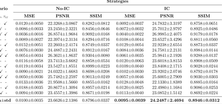
3.3.2 Effect of Implicit Conditioning (IC) . . . 29

3.3.3 Reconstruction Error in Other Planes . . . 31

3.4 Multimodal Synthesis (MIMO) . . . 31

4 Conclusions and Future Work 38

List of Tables

Table 2.1 Patient images used for testing from BraTS2018 HGG and LGG cohorts. 16

Table 3.1 Comparison between P2P, pGAN and MI-GAN. Values in boldface

represent best performance values. Reported values are mean± std. . 22

Table 3.2 Comparison with unimodal method REPLICA and multimodal method

MM-Synthesis. The reported values are mean squared error (MSE). Boldface values represent lowest values of the three methods for a par-ticular scenario. . . 25 Table 3.3 Quantitative experiments testing three different imputation methods

z ∈ {average, noise, zeros}, as well as two training strategies

curricu-lum learning (CL) and random sampling (RS). The combination z =

zeros and curriculum learning based training performs the best in terms

of MSE and PSNR, while z = zeros and random sampling performs

slightly better in SSIM. Bit strings 0001 to 1110 denote absence (0) or presence (1) of sequences in order T1,T2,T1c,T2f lair respectively. . . 28

Table 3.4 Quantitative results for evaluating effectiveness of implicit conditioning (IC) based training strategy. . . 30 Table 3.5 Results for Mann-Whitney U statistical test on 5 test patients from

LGG cohort. p-values from two tests (axial vs coronal and axial vs sagittal) are reported. . . 31

Table 3.6 Performance on BraTS2018 High Grade Glioma (HGG) Cohort . . . 32

Table 3.7 Performance on BraTS2018 Low Grade Glioma (LGG) Cohort . . . . 33

Table 3.8 MM-GAN performance variation with respect to number of sequences missing for HGG and LGG cohort. . . 36

List of Figures

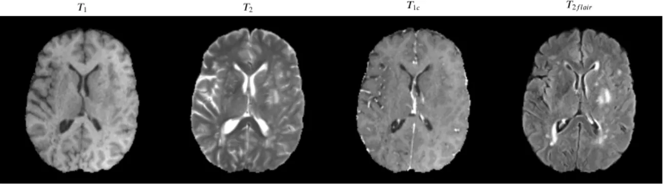
Figure 1.1 Common MR sequences acquired for a patient. Axial slices from a

high grade glioma (HGG) patient from BraTS2018 are shown. . . . 1

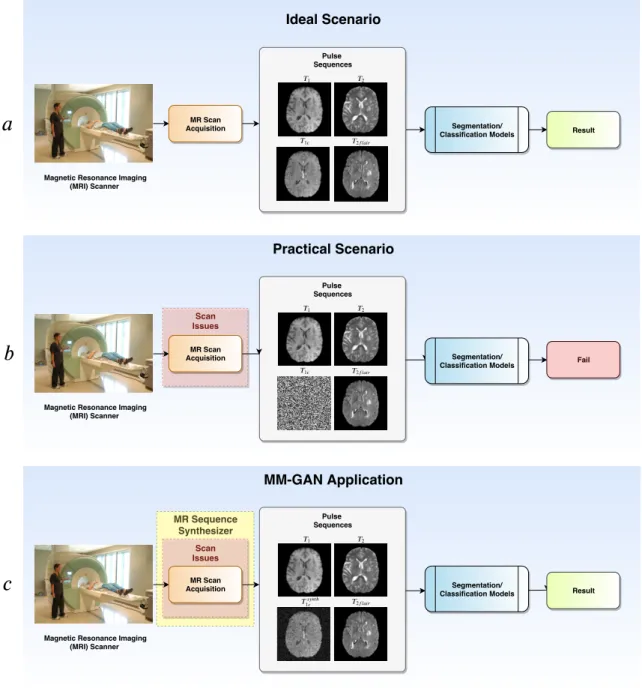
Figure 1.2 Illustration of scenarios where MR pulse sequences may be missing. (a) shows an ideal scenario where MR scan is acquired consisting of all the required sequences (T1, T2, T1c, T2f lair). (b) shows

prac-tical scenario where the scan may be interrupted or the sequences get missing due to other reasons, leading to downstream deployed algorithms to fail due to their hard reliance on the particular set of sequences. (c) a valid use-case where MR pulse sequence synthesizer like MM-GAN may be inserted in the pipeline to generate missing sequences, and allowing the deployed downstream algorithms to still function without failing. . . 3

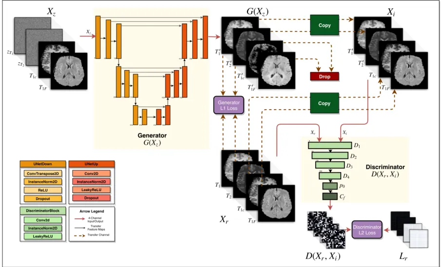
Figure 2.1 Proposed multimodal generative adversarial network (MM-GAN)

training process. The generator is a UNet architecture, while the dis-criminator is a PatchGAN architecture with L2 loss (least squares GAN). The green “Copy” blocks transfer the input channels as is to its output, while the red “Drop” block deletes its input channels. The generator L1 loss is computed only between the synthesized versions of the missing sequences (here T1 and T2). The discriminator takes

XrandXias input and produces a 4-channel 2D output representing

whether eachN ×N patch inXi is either fake or real. . . 10

Figure 3.1 Qualitative results for P2P, pGAN, and MI-GAN. Left subfigure

(columns (a) through (d)) visualize the performance of three mod-els in synthesis of T1 sequence. The second subfigure (columns (e) through (h)) show synthesized T2 sequences for each of the tested models. Red arrows indicate areas where tumor regions were present, and successfully synthesized by MI-GAN in bothT1 and T2 synthesis. 23

Figure 3.2 Qualitative results fromT2f lairsynthesis experiments with ISLES2015

dataset. The order of scenario bit-string isT1,T2, DW,T2f lair, where

a zero (0) represents missing sequence, while a one (1) represents an available sequence. We note that the presence of multiple sequences (scenario 1110) qualitatively matches the closest to the ground truth, with sharp boundaries between white and grey matter, as well as less blurring artifacts compared to scenarios with two or just one avail-able sequences. Patient images shown here are from VSD ID 70668 from ISLES2015 SISS cohort. . . 26 Figure 3.3 Qualitative results from the multimodal synthesis experiments with

BRaTS2018 dataset. Each row corresponds to a particular sequence (row names on the left in orderT1,T2,T1candT2f lair). Columns are

indexed at the bottom of the figure by alphabets (a) through (h), and have a column name written on top of each slice. Column names are 4-bit strings where a zero (0) represents missing sequence that was synthesized, and one (1) represents presence of sequence. Column (a) of each row shows the ground truth slice, and the subsequent columns ((b) through (h)) show synthesized versions of that slice in different scenarios. The order of scenario bit-string is T1, T2, T1c,

T2f lair. For instance, the string 0011 indicates that sequencesT1 and

T2 were synthesized from T1c and T2f lair sequences. Patient images

shown here are fromBrats18_CBICA_AAP_1 from HGG cohort. 34

Figure 3.4 Illustration of MM-GAN filling up parts in the scan that are orig-inally missing in the ground truth. Red arrow shows the top part of brain that is missing, and is synthesized in all scenarios. Blue ar-row highlights the high-frequency details that are missing in ground truth, but are synthesized in most images. We also notice that when all sequences are present, the T2f lair synthesis is the most accurate

with respect to the pathology visible in the frontal cortex. The order of scenario bit-string is T1, T2, T1c, T2f lair. Patient images shown

Chapter 1

Introduction

1.1

Motivation and Context

Medical imaging forms the backbone of the modern healthcare systems, providing means to assess, diagnose, and plan treatments for a variety of diseases. Imaging techniques like computed tomography (CT), magnetic resonance imaging (MRI), X-Rays have been in use for over many decades. Magnetic resonance imaging (MRI) out of these is particularly in-teresting in the sense that a single MRI scan is a grouping of multiple pulse sequences, each of which provides varying tissue contrast views and spatial resolutions, without the use of radiation. These sequences are acquired by varying the spin echo and repetition times during scanning, and are widely used to show pathological changes in internal or-gans and muscoskeletal system. Some of the commonly acquired sequences areT1-weighted,

T2-weighted, T1-with-contrast-enhanced (T1c), and T2-fluid-attenuated inversion recovery (T2f lair), though there exist many more [1]. The common sequences are shown in Figure

1.1.

A combination of sequences provide both redundant and complimentary information to the physician about the imaged tissue, and certain diagnosis are best performed when a particular sequence is observed. For example, T1 and T2f lair sequences provide clear

delin-2

1 2 1

Figure 1.1: Common MR sequences acquired for a patient. Axial slices from a high grade glioma (HGG) patient from BraTS2018 are shown.

eations of the edema region of tumor in case of glioblastoma,T1cprovides clear demarcation

of enhancing region around the tumor used as an indicator to assess growth/shrinkage, and

T2f lair sequence is used to detect white matter hyperintensities for diagnosing vascular

dementia (VD) [2].

In clinical settings, however, it is common to have MRI scans acquired using varying protocols, and hence varying sets of sequences per patient. Sequences which are routinely acquired may be unusable or missing altogether due to scan corruption, artifacts, incorrect machine settings, allergies to certain contrast agents and limited available scan time [3–5]. This phenomenon is problematic for many downstream data analysis pipelines that assume presence of a certain set of pulse sequences to perform their task. For instance, most of the segmentation methods [6–10] proposed for brain MRI scans depend implicitly on the availability of a certain set of sequences in their input in order to perform the task. Most of these methods are not designed to handle missing inputs, and hence may fail in the event where some or most of the sequences may be absent. This is also illustrated in Figure 1.2.

Modifying existing pipelines in order to handle missing sequences is hard, and may lead to performance degradation. Also, the option of redoing a scan to acquire the miss-ing/corrupted sequence is impractical due to the expensive nature of the acquisition, longer wait times for patients with non-life-threatening cases, need for registration between old and new scans, and rapid changes in anatomy of area in-between scan times due to highly active abnormalities such as glioblastoma. Hence there is a clear advantage in retrieving any missing sequence or an estimate thereof, without having to redo the scan or changing the downstream pipelines.

To this end, we propose a multi-modal generative adversarial network (MM-GAN) which is capable of synthesizing missing sequences by combining information from all available se-quences. The proposed method exhibits the ability to synthesize, with high accuracy, all the required sequences which are deemed missing in a single forward pass through the network. The term “multi-modal” simply refers to the fact that the GAN can take multiple-modalities of available information as input, which in this case represents different pulse sequences. Similar to the input being multi-modal, our method generates multi-modal output contain-ing synthesized versions of the misscontain-ing sequences. Since most of the downstream analysis pipelines commonly target C = 4 pulse sequences S = {T1, T1c, T2, T2f lair} as their

in-put [7, 11, 12], we design our method around the same number of sequences, although we note that our method can be generalized to any number C and set S of sequences. The input to our network is a 4-channel (corresponding to C = 4 sequences) 2D axial slice, where a zero image is imputed for channels corresponding to missing sequences. The output of the network is a 4-channel 2D axial slice, in which the originally missing sequences are synthesized by the network.

Magnetic Resonance Imaging (MRI) Scanner  MR Scan Acquisition Pulse  Sequences 2 1 1 2 Segmentation/

Classification Models Result

Ideal Scenario

Magnetic Resonance Imaging (MRI) Scanner  MR Scan Acquisition Pulse  Sequences 2 1 1 2 Fail Practical Scenario Scan Issues

Magnetic Resonance Imaging (MRI) Scanner  MR Scan Acquisition Pulse  Sequences 2 ℎ 1 1 2 MM-GAN Application Scan Issues MR Sequence Synthesizer Result Segmentation/ Classification Models Segmentation/ Classification Models

Figure 1.2: Illustration of scenarios where MR pulse sequences may be missing. (a) shows an ideal scenario where MR scan is acquired consisting of all the required sequences (T1,T2,T1c,

T2f lair). (b) shows practical scenario where the scan may be interrupted or the sequences get

missing due to other reasons, leading to downstream deployed algorithms to fail due to their hard reliance on the particular set of sequences. (c) a valid use-case where MR pulse sequence synthesizer like MM-GAN may be inserted in the pipeline to generate missing sequences, and allowing the deployed downstream algorithms to still function without failing.

1.2

Related Work

There has been an increased amount of interest in developing methods for synthesizing MR pulse sequences [2, 5, 13–26]. We present a brief overview of previous work in this field by covering them in two sections: Unimodal, where both the input and output of the system is a single pulse sequence (one-to-one); and multimodal, where methods are able to leverage multiple input sequences to synthesize a single to-one) or multiple sequences (many-to-many).

1.2.1 Unimodal Synthesis

In unimodal synthesis (one-to-one), a common strategy includes building an atlas or a database that maps intensity values between given sequences. Jog et al. [15] used a bagged ensemble of regression trees trained from an atlas. The training data (A1,A2) consisted of multiple image patches A₁ around a voxel i in a source sequence, and a single intensity value at the same voxel in a target sequence, as A2. The use of image patches to predict the intensity value of a single voxel in output sequence allows representing many-to-many relationship between intensity values of input and target sequences. Ye et al. [14] propose an inverse method, which performs a local patch-based search in a database for every voxel in the target pulse sequence. Once the patches are found, they are “fused” together using a data-driven regularization approach. Another atlas based method was proposed in [19] whereT2 whole-head sequence (including skull, eyes etc.) is synthesized from the available

T1 images. The synthesized T2 sequence is used to correct distortion in diffusion-weighted MR images by using it as template for registration, in the absence of a real T2 sequence. Yawen et al. [20] leverage joint dictionary learning (JDL) for synthesizing any unavailable MRI sequence from available MRI data. JDL is performed by minimizing the inconsistency between statistical distributions of the dictionary codes for input MRI sequences while preserving the geometrical structure of the input image.

Supervised machine learning and deep learning (DL) based methods have also been employed in sequence synthesis pipelines. A 3D continuous-valued conditional random field (CRF) is proposed in [18] to synthesize T2 images from T1. The synthesis step is encoded as a maximum a-posterior (MAP) estimate of Gaussian distribution parameters built from a learnt regression tree. Nguyen et al. [27] was one of the first to employ DL in the form of location-sensitive deep network (LSDN) for sequence synthesis. LSDN predicts the intensity value of the target voxel by using voxel-centered patches extracted from an input sequence. The network models the responses of hidden nodes as a product of feature and spatial responses. Similarly, Bowleset et al. [2] generate “pseudo-healthy” images by performing voxel-wise kernel regression instead of deep networks to learn local relationships between intensities inT1 and T2f lair sequences of healthy subjects. Since most of the methods were

input sequence, Sevetlidis et al. [21] proposed an encoder-decoder style deep neural network trained layer-wise using restricted Boltzmann machine (RBM) based training. The method utilized global context of the input sequence by taking a full slice as input. Recently, Jog et al. [22] propose a random forest based method that learns intensity mapping between input patches centered around a voxel extracted from a single pulse sequence, and the intensity of corresponding voxel in target sequence. The method utilized multi-resolution patches by building a Gaussian pyramid of the input sequence. Yu et al. [26] propose a unimodal GAN architecture to synthesize missing pulse sequences in a one-to-one setting. The approach uses an edge detection module that tries to preserve the high-frequency edge features of the input sequence, in the synthesized sequence. Recently, Ul Hassan Dar et al. [28] propose to use a conditional GAN to synthesize missing MR pulse sequences in a unimodal setting for two sequencesT1 and T2.

1.2.2 Multimodal Synthesis

Multimodal synthesis has been a relatively new and unexplored avenue in MR synthesis literature. One of the first multi-input, single-output (many-to-one) method was proposed by Jog et al. [16]; a regression based approach to reconstructT2f lairsequence using combined

information from T1,T2, and proton density (PD) sequences. Reconstruction is performed by a bagged ensemble of regression trees predicting theT2f lair voxel intensities. Chartsias et

al. [5] were one of the first to propose a multi-input, multi-output (many-to-many) encoder-decoder based architecture to perform many-to-many sequence synthesis, although their multimodal method is tested only using a single-output (T2f lair) (many-to-one setting).

Their network is trained using a combination of three loss functions, and uses a feature fusion step in the middle that separates the encoders and decoders. Olut et al. [23] present a GAN based framework to generate magnetic resonance angiography (MRA) sequence from available T1, and T2 sequences. The method uses a novel loss function formulation, which preserves and reproduces vascularities in the generated images. Although for a different application, Mehta et al. [24] proposed a multi-task, multi-input, multi-output 3D CNN that outputs a segmentation mask of the tumor, as well as a synthesized version of T2f lair

sequence. The main aim remains to predict tumor segmentation mask from three available sequencesT1,T2, andT1c, and no quantitative results forT2f lair synthesis usingT1,T2, and

T1c are provided.

Though all the methods discussed above propose a multi-input method, none of the methods have been proposed to synthesize multiple missing sequences (multi-output), and in one single pass. All three methods [16], [5], and [24] synthesize only one sequence (either

T2f lair or T2, many-to-one setting) in the presence of varying number of input sequences, while [23] only synthesizes MRA using information from multiple inputs (many-to-one). Although the work presented in [23] is close to our proposed method, theirs is not a truly multimodal network (many-to-many), since there is no empirical evidence that their method

will generalize to multiple scenarios. Similarly, the framework proposed in [5] can theoreti-cally work in a many-to-many setting, but no empirical results are given to demonstrate its scalability and applicability in a variety of different scenarios, as we do in this work. The authors briefly touch upon this by adding a new decoder to already trained many-to-one network, but do not explore it any further. To the best of our knowledge, we are the first to propose a method that is capable of synthesizing multiple missing sequences using a combination of various input sequences (many-to-many), and demonstrate the method on the complete set of scenarios (i.e., all combinations of missing sequences).

The main motivation for most synthesis methods is to retain the ability to meaning-fully use some downstream analysis pipelines like segmentation or classification despite the partially missing input. However, there have been efforts by researchers working on those analysis pipelines to bypass any synthesis step by making the analysis methods themselves robust to missing sequences. Most notably, Havaei et al. [3] and Varsavsky et al. [4] provide methods for tumor segmentation using brain MRI that are robust to missing sequences [3], or to missing sequence labels [4]. Although the methods bypass the requirement of hav-ing a synthesis step before actual downstream analysis, the performance of these robust versions of analysis pipelines often do not match the state-of-the-art performance of other non-robust methods in the case when all sequences are present. This is due to the fact that the methods not only have to learn how to perform the task (segmentation/classification) well, but also to handle any missing input data. This two-fold objective for a single network raises a trade-off between robustness and performance.

1.3

Thesis Contributions

The following are the key contributions of this work:

1. We propose the first multi-input multi-output MR pulse sequence synthesizer capable of synthesizing missing pulse sequences using any combination of available sequences as input without the need for tuning or retraining of models, in a many-to-many setting.

2. The proposed method is capable of synthesizing any combination of target missing sequences as outputin one single forward pass, and requires only a single trained model for synthesis. This provides significant savings in terms of computational overhead during training time compared to training multiple models in the case of unimodal and multi-input single-output methods.

3. We propose to use implicit conditioning (IC), a combination of three design choices, namely imputation in place of missing sequences for input to generator, sequence-selective loss computation in the generator, and sequence-sequence-selective discrimination.

We show that IC improves overall quantitative synthesis performance of generator compared to the baseline approach without IC.

4. To the best of our knowledge, we are the first to incorporate curriculum learning based training for GAN by varying the difficulty of examples shown to the network during training.

5. Through experiments, we show that we outperform both the current state-of-art in unimodal (pGAN [28]), as well as the multi-input single-output synthesis (REPLICA [22] and MM-Synthesis [5]) method. We also set up new benchmarks on a complete set of scenarios using the BraTS2018 dataset.

1.4

Thesis Outline

The rest of the thesis is organized as follows: Chapter 2 presents detailed description of the proposed method, along with implementation details, datasets used, as well as outlines experimental setup for the current work. Chapter 3 discusses the results and observations for the proposed method, and finally the thesis is concluded in Chapter 4.

Chapter 2

Methodology

2.1

Background

Generative adversarial networks (GANs) were first proposed by Goodfellow et al. [29] in order to generate realistic looking images. A GAN is typically built using a combination of two networks: generator (G) and discriminator (D). The generator network is tasked with generating realistic data, typically by learning a mapping from a random vector z to an imageI:

G :z→I, (2.1)

whereI is said to belong to the generator’s distribution pG.

The discriminator:

D:I →t (2.2)

maps its inputI to a target labelt∈ {0,1}, wheret= 0 ifI ∈pG, i.e. a fake image generated

by G and t = 1 if I ∈ pr where pr is the distribution of real images. A variant of GANs,

called conditional-GAN (cGAN) [30], proposes a generator that learns a mapping from a random vectorz and a class labely to an output image I:

G: (z, y)→I, I∈pG (2.3)

Another variant of cGAN called Pix2Pix [31] develops a GAN in which the generator learns a mapping from an input image x∈pr to output image I ∈pG,G :x →I, and the

discriminator learns a mapping from two input images, x1 and x2, to T,D: (x1, x2)→ T.

x1 and x2 may belong to eitherpr (real) or pG (fake). The output T in this case is a not a

single class label, but a binary prediction tensor representing whether eachN×N patch in the input image is real or fake [31].

A GAN is trained in an adversarial setting, where the generator (parameterized by θG)

is trained to synthesize realistic output that can ”fool” the discriminator into classifying them as real, and the discriminator (parameterized by θD) is trained to accurately

distin-guish between real data and fake data synthesized by the generator. GAN input/outputs can be images [31], text [32] or even music [33]. Both the generator and discriminator act as adversaries to each other, hence the training formulation forces both networks to contin-uously get better at their tasks. GANs found tremendous success in a variety of different tasks, ranging from face-image synthesis [34], image stylization [35], future frame predic-tion in videos [36], text-to-image synthesis [32] and synthesizing scene images using scene attributes and semantic layout [37]. GANs have also been utilized in medical image analysis [38], particularly for image segmentation [39–41], normalization [42], synthesis [23, 26, 28] as well as image registration [43].

UNetDown UNetUp DiscriminatorBlock zT1 zT2 T1c T1F T2 T1c T1F T′ 1 T′ 2 T′ 1c T′ 1F T′ 1 T′ 2 T1c T1F Drop Copy Discriminator L2 Loss

X

X

X

D( , )

X

X

L

G( )

X

Figure 2.1: Proposed multimodal generative adversarial network (MM-GAN) training process. The generator is a UNet architecture, while the discriminator is a PatchGAN architecture with L2 loss (least squares GAN). The green “Copy” blocks transfer the input channels as is to its output, while the red “Drop” block deletes its input channels. The generator L1 loss is computed only between the synthesized versions of the missing sequences (here T1 and T2). The discriminator takesXr and Xi as input and produces a 4-channel

2D output representing whether eachN ×N patch inXi is either fake or real.

2.2

Proposed Method

We propose a variant of Pix2Pix architecture [31] called Multi-Modal Generative Adver-sarial Network (MM-GAN) for the task of synthesizing missing MR pulse sequences in a single forward pass while leveraging all available sequences. The following subsections would outline the detailed architecture of our model.

2.2.1 Generator

The generator of the proposed method is a UNet [44], which has proven useful in a variety of segmentation and synthesis tasks due to its contracting and expanding paths in the form of encoder and decoder subnetworks. The architecture is illustrated in Figure 2.1. The convolution kernel sizes for each layer in the generator is set to 4×4. The generator network is a combination of UNetUpand UNetDownblocks. The input to the generator is a 2D axial slice from a patient scan withC= 4 channels representing four pulse sequences, and spatial size of 256×256 pixels. The network is designed with a fixed input size of 4-channels, where channel C= 0,1,2,and 3 corresponds toT1,T2,T1c, and T2f lair, respectively.

In order to synthesize missing sequences, the channels corresponding to each missing sequence are imputed with zeros. The imputed version (along with the real sequences) becomes the input to the generator and is represented byXz. For instance, if sequencesT1 and T2 are missing, channelsC= 0 and C= 1 in the input image are imputed with a zero image of size 256×256. The output of the generator is given by G(Xz|θG) and is of the

same size as the input. Due to design, the generator always outputs 4 channels, however, as we outline in the subsequent text the output channels corresponding to the existing real sequences are not used for loss computation and are replaced with the real sequences before relaying them as input to the discriminator. During training the ground truth image Xr,

short for “real”, which is of the same size asXz contains all ground truth sequences at their

respective channel indices. We use the term “image” for a single 2D slice with 4 channels. MM-GAN observes both an input image and imputed zeros z in the form of Xz, in

contrast to vanilla Pix2Pix where the generator is conditioned just by an observed imagex. The reasons behind this design choice are discussed in subsection 2.2.3. We also investigate different imputation strategies in subsection 3.3.1, and found that zero based imputation performs the best quantitatively.

To optimizeθG, our generator adopts the general form of the generator loss in Pix2Pix,

which is a combination of a reconstruction lossL₁ and an adversarial lossL₂ used to train the generator to fool the discriminator, i.e.

θ_G∗ = arg min

θG

λL₁(G(Xz|θG), Xr)+

(1−λ)L2(D(Xi, Xr|θD), Lar).

To calculate L₁, we select synthesized sequences from G(Xz|θG), that were originally

missing, and compute the L1 norm of the difference between the synthesized versions of the sequence and the available ground truth from Xr. Mathematically, given the set K

containing the indices of missing sequences (e.g. K ={0,2} when T1 and T1c are missing)

in the current input, we calculateL1 only for the sequences that are missing (k= 0,2), and sum the values.

To calculate L₂, we compute the squared L2 norm of the difference between the dis-criminator’s predictionsD(Xi, Xr|θD)) and a dummy ground truth tensorLar of the same

size as the output of D. In order to encourage the generator to synthesize sequences that confuse or “fool” the discriminator into predicting they are real, we set all entries of Lar to

ones, masquerading all generated sequences as real.Xi is introduced in the next section.

The choice of L1 as a reconstruction loss term for the generator is motivated by its ability to prevent too much blurring in the final synthesized sequences, as compared to using an L2 loss (similar to [31]).

2.2.2 Discriminator

We use the PatchGAN architecture [31] for the discriminator part of our MM-GAN. Patch-GAN architecture learns to take into account the local characteristics of its input, by pre-dicting a real/fake class for every N ×N patch of its input, compared to classic GANs where the discriminator outputs a single real/fake prediction for the whole input image. This encourages the generator to synthesize images not just with proper global features (shape, size), but also with accurate local features (texture, distribution, high-frequency details). In our case we set N = 16.

The discriminator is built using four blocks followed by a zero padding layer and a final convolutional layer (Figure 2.1). The convolutional kernel sizes, stride and padding is identical to the values used in the generator (subsection 2.2.1). Due to the possibility of having a varying number of sequences missing, instead of providing just the synthesized sequences and their real counterparts as input to the discriminator, we first create a modified version of G(Xz|θG) by dropping the reconstructed sequences that were originally present,

and replacing them with the original sequences fromXr. The modified version of G(Xz|θG)

is represented byXi, short for “imputed”. The input to the discriminator is a concatenation

of Xi and Xr. This is also illustrated in Figure 2.1.

The discriminator is trained to output a 2D patch of size 16×16 pixels, with 4 channels corresponding to each sequence. In order to supervise the discriminator during training, we use a 4-channel 2D image based target, in which each channel corresponds to a sequence. More specifically, given missing sequences K (e.g., K = {0,2}, T1 and T1c missing), the

Lk_r =    0.0 (fake) ifk∈K 1.0 (real) otherwise (2.5)

Note thatLk_r is a 2D tensor of size 16×16 (since each 256×256 image is divided into 16×16 patches) yet the assignment of 0.0 or 1.0 represents an assignment to the whole 16×16

Lk_r tensor (since the whole image is either real or fake and not patch-specific). This is also illustrated in Figure 2.1.

Between the output of discriminatorD(Xi, Xr|θD) andLr, an L2 loss is computed. The

final discriminator loss becomes:

θ∗_D= arg min

θD

L₂(D(Xr, Xr|θD), Lar)

+L₂(D(Xr, Xi|θD), Lr).

(2.6)

This is equivalent to a least-squares GAN since the loss function incorporates an L2 loss.

2.2.3 Implicit conditioning

Due to the inherent design of deep learning architectures, the input as well as output of a convolutional neural network model has to have a fixed channel dimension. In our use case however, both the input and output channel dimensions vary (since the number of available sequences can vary).

In order to address this problem, we propose a combination of three design choices, which we collectively refer to as implicit conditioning (IC). In IC, the varying input channels prob-lem is solved by imputing a fixed value (zeros) to the input channels where the sequences are missing. For the problem of generator output size being fixed in channel dimension, one possible approach can be to synthesize all four input sequences. The loss function can be calculated between four ground truth sequences, and the four synthesized sequences. How-ever, this poses a challenge for the generator, as its burdened with generating all sequences, including the reconstruction of the ones that were provided as input. In order to address this, we proposed selective loss computation inG, where the loss is only calculated between the ground truth sequences that were missing, and the corresponding output channels of the generators. In conjunction, we also propose selective discrimination inD, which ensured stability during training by preventing the discriminator from overpowering the generator. We also show that IC-based training outperforms the baseline training methodology of gen-erating and penalizing inaccurately synthesizing all sequences (subsection 3.3.2). The design choices are individually summarized below.

2.2.3.1 Input Imputation

The input Xz of the generator always contains an imputed value (z = zeros) in place of

the missing sequences which acts as a way to condition the generator and informs which sequence(s) to synthesize.

2.2.3.2 Selective Loss Computation in Generator (G)

In conjunction, the L1(G) loss that is computed only between the synthesized sequences for the generator, and then backpropagated, allows the generator to align itself towards only synthesizing the actual missing sequences properly while ignoring the performance in synthesizing the ones that were already present.

2.2.3.3 Selective Discrimination in Discriminator (D)

Imputing real sequences at the generator output (i.e.Xi) before providing it as discriminator

input forces the discriminator to accurately learn to delineate only between the synthesized sequences and their real counterparts. Since the generator loss function also has a term that tries to fool the discriminator, this allows selective backpropagation into the generator where it is penalized only for incorrectly synthesizing the missing sequences, and not for incorrectly synthesizing the sequences that were already present. This relieves the generator of the difficult task of synthesizing all sequences in the presence of some sequences.

2.2.4 Curriculum Learning

In order to train our proposed method we use a curriculum learning (CL) [45] based ap-proach. In CL based training, the network is initially shown easier examples followed by increasingly difficult examples as the training progresses. We hypothesized that CL can ben-efit in training of MM-GAN due to an ordering in the level of difficulty across the various scenarios that the network has to handle. If some cases are “easier” than others, it might be useful if the easier cases are shown first to the network in order to allow the network to effectively learn when ample supervision is available. As the network trains, “harder” cases can be introduced so that the network adapts without diverging.

In our work, scenarios with 1 sequence missing are considered “easy”, followed by a “moderate” set of scenarios with 2 missing sequences, and lastly, the scenarios with 3 missing sequences are considered “hard”. We adopted this ordering in our work, and showed the network easier examples first, followed by moderate and finally hard examples. After a threshold of 30 epochs, we show every scenario with uniform probability.

2.3

Experimental Setup

In this section we describe different aspects of the experiments that are performed in this work.

2.3.1 Datasets

In order to validate our method we use brain MRI datasets from two sources, namely the Ischemic Stroke Lesion Segmentation Challenge 2015 (ISLES2015) [46] and the Multimodal Brain Tumor Segmentation Challenge 2018 (BraTS2018) [47].

2.3.1.1 Ischemic Stroke Lesion Segmentation Challenge 2015

ISLES2015 dataset is a publicly available database with multi-spectral MR images [46]. We choose the sub-acute ischemic stroke lesion segmentation (SISS) cohort of patients, which contains 28 training and 36 testing cases. The patient scans are skull stripped using BET2 [48], and resampled to an isotropic resolution of 1 mm3. Each scan consists of four sequences namely T1,T2, DWI, and T2f lair, and are rigidly co-registered to the T2f lair

se-quence using elastix tool-box [49]. More information about the preprocessing steps can be found in the original publication [46]. We use 22 patients from the SISS training set for experiments.

2.3.1.2 Brain Tumor Segmentation Challenge 2018

BraTS2018 consists of a total of 285 patient MR scans acquired from 19 different institu-tions, divided into two cohorts: glioblastoma/high grade glioma (GBM/HGG) and low grade glioma (LGG). The patient scans contains four pulse sequenceT1,T2,T1c, andT2f lair. All

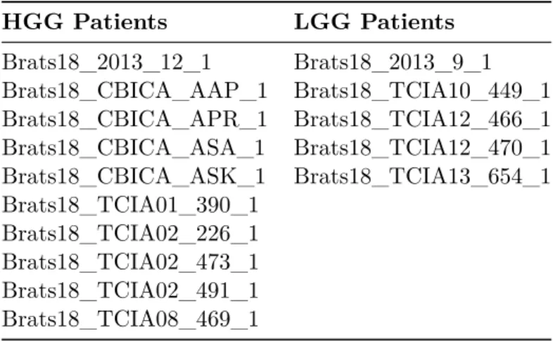
scans are resampled to 1 mm3 isotropic resolution using a linear interpolator, skull stripped, and co-registered with a single anatomical template using rigid registration model with mu-tual information similarity metric. Detailed preprocessing information can be found in [47]. In order to demonstrate our method’s ability in synthesizing sequences with both high grade and low grade glioma tumors present, we use a total of 210 patients from HGG and 75 patients from LGG cohort. 195 patients are reserved for training for HGG cohort, while 65 are used for training in LGG experiments. For validation, we use 5 patients for both HGG and LGG cohorts. In order to test our trained models, we use 10 patients from HGG cohort (due to larger data available), while we report results using 5 patients for LGG cohort as testing. To enable direct comparisons by future works, we release the list of patient images used as test set throughout this study in the Table 2.1. Patients other than those specified in Table 2.1 are used for training.

Table 2.1: Patient images used for testing from BraTS2018 HGG and LGG cohorts. HGG Patients LGG Patients Brats18_2013_12_1 Brats18_2013_9_1 Brats18_CBICA_AAP_1 Brats18_TCIA10_449_1 Brats18_CBICA_APR_1 Brats18_TCIA12_466_1 Brats18_CBICA_ASA_1 Brats18_TCIA12_470_1 Brats18_CBICA_ASK_1 Brats18_TCIA13_654_1 Brats18_TCIA01_390_1 Brats18_TCIA02_226_1 Brats18_TCIA02_473_1 Brats18_TCIA02_491_1 Brats18_TCIA08_469_1 2.3.2 Preprocessing

Each patient scan is normalized by dividing each sequence by its mean intensity value. This ensures that distribution of intensity values is preserved [5]. Normalization by mean is less sensitive to high or low intensity outliers as compared to min-max normalization procedures, which can be greatly exacerbated by the presence of just a single high or low intensity voxel in a sequence. This is especially common in the presence of various pathologies, like tumors as in BraTS2018 datasets, which tend to have very high intensity values in some sequences (T2, T2f lair) and recessed intensities in others (T1, T1c). In practice, we observed this for

BraTS2018 HGG cohort, where some voxels had an unusually high intensity value due to a pathology. On performing min-max normalization to scale intensities between [0,1], we found that the presence of very high intensity voxel squashed the pixel range to always lie very close to zero. This artificially bumped the performance numbers for the generator since most voxels lied close to zero, and hence the generator could synthesize images with intensity values close to zero, and achieve a low L1 score easily. On the other hand, mean normalization was relatively unaffected due to a large number of voxels in a defined range ( 0-4000). The mean value was not strongly affected by the presence of one or more high/low intensity voxels.

We also tested the method internally with zero mean and unit variance based standard-ization, and found the results to be at par with mean normalization. In order to crop out the brain region from each sequence, we calculate the largest bounding box that can accommo-date each brain in the whole dataset, and then use the coordinates to crop each sequence in every patient scan. The final cropped size of a single patient scan with all sequences contains 148 axial slices of size 194×155. Each slice in every sequence is resized to a spatial resolution of 256×256, using bilinear interpolation, in order to maintain compatibility with UNet architecture of the generator.

We note that avoiding resampling twice (once during registration performed by the original authors of the dataset, and once during resampling to 256×256 in this work) may preserve some information in the scans that may otherwise be lost. However, it is a necessary preprocessing step in order to maintain compatibility with various network architectures that we utilize, which includes inherent assumptions that the input size would be a power of two to allow successive contracting and expanding steps used in many encoder-decoder style architectures. In order to fully avoid the second resampling step (to 256×256 in this work), a different network architecture may be used without the encoder-decoder setup, though the performance of those networks may not be at par with the modern encoder-decoder style networks as established in synthesis field [28, 31, 50]

2.3.3 Benchmark Methods

We compare our method with three competing methods, one unimodal and two multimodal. The unimodal (single-input, single-output, one-to-one) method we compare against is pGAN [28], while the multimodal (many-to-one) models being REPLICA [22] (in a multi-input setting), and that of Chartsias et al. [5], called MM-Synthesis hereafter. Both pGAN and MM-Synthesis were recently published (2019 and 2018), and they outperform all other methods before them (MM-Synthesis outperforms LSDN [27], Modality Propagation [14], and REPLICA [22], while pGAN outperforms both REPLICA and MM-Synthesis in one-to-one synthesis). To the best of our knowledge, we did not find any other methods that claimed to outperform either pGAN or MM-Synthesis, and so decided to evaluate our method against them.

For comparison with pGAN [28], we reimplement the method using the open source code provided with the publication, and train both pGAN and our method on a randomly chosen subset of data from BRATS2018 LGG cohort. We also compare with a standard baseline which is a vanilla Pix2Pix [31] model trained and tested in a one-to-one setting. For our multimodal (many-to-one) experiments, we report mean squared error (MSE) results for both REPLICA and MM-Synthesis directly from [5], as we recreate the exact same testbed for comparison with MM-GAN, as used in MM-Synthesis. We adopt the same testing strategy (5-fold cross validation), database (ISLES2015), and scenarios (7 scenarios where T2f lair is always missing and is the only one that is synthesized). As highlighted

in [5], the multi-input version of REPLICA required seven models each for each of the seven valid scenarios in many-to-one setting synthesizing T2f lair sequence. MM-Synthesis

and our proposed MM-GAN only required a single multimodal (many-to-one) network which generalized to all seven scenarios.

For our final extended set of experiments, we demonstrate the effectiveness of our method in a multi-input multi-output (many-to-many) setting, where we perform testing on the HGG and LGG cohorts of BRaTS2018 dataset for which we report results of all 14 valid scenarios (=16−2, as scenario when all sequences are missing/present are invalid for our

ex-periments) instead of just 7. The results showcase our method’s generalizability on different use-cases with varying input and output subsets of sequences, and different difficulty levels. We use a fixed order of sequences (T1,T2,T1c,T2f lair) throughout this thesis, and represent

each scenario as a 4-bit string, where a zero (0) represents the absence of a sequence at that location, while a one (1) represents its presence.

2.3.4 Training and Implementation Details

In order to optimize our networks, we use Adam [51] optimizer with learning rateη = 0.0002,

β1 = 0.5 andβ2= 0.999. Both the generator and discriminator networks are initialized with weights sampled from a Gaussian distribution withµ= 0, σ= 0.02.

We perform four experiments, first for establishing that multi-input synthesis is better than single-input (many-to-one vs one-to-one respectively), second for T2f lair synthesis

us-ing multiple inputs (many-to-one) (called MISO, short for multi-input sus-ingle-output) usus-ing ISLES2015 dataset to compare with REPLICA and MM-Synthesis. The third set of experi-ments encompasses validation of multiple key components proposed throughout this thesis, in terms of their contribution towards overall network performance. We test different impu-tation strategies (z ={average, noise, zeros}), as well as the effect of curriculum learning (CL) and implicit conditioning (IC). The final set of experiments pertain to multimodal synthesis (MIMO, short for multi-input multi-output), which sets a new benchmark for many-to-many synthesis models using BraTS2018 HGG and LGG cohorts. We refer to the second and fourth experiments as MISO and MIMO, respectively, hereafter. We use a batch size of 4 slices to train models, except for MISO, where we use batch size of 2. We train the models for 30 epochs in MISO and 60 epochs for MIMO sets of experiments, with no data augmentation.

We choose λ= 0.9 for the generator loss given in equation 2.4, while we multiply the discriminator loss by 0.5 which essentially slows down the rate at which discriminator learns compared to generator. During each epoch, we alternate between a single gradient descent step on the generator, and one single step on the discriminator.

For our MIMO experiments, we use the original PatchGAN [31] discriminator. However for our MISO experiments, due to lack of training data, we used a smaller version of the PatchGAN discriminator with just two discriminator blocks, followed by a zero padding and final convolution layer. Also, random noise was added to both Xr and Xi inputs of

the discriminator in MISO experiments. This was done to reduce the complexity of the dis-criminator to prevent it from overpowering the generator, which we observed when original PatchGAN with no noise imputation in its inputs was used for this set of experiments. The generator’s final activation was set to ReLU for MIMO and linear for MISO experiments due to the latter having negative intensity values for some patients.

For our implementation we used Python as our main programming language. We imple-mented Pix2Pix architecture in PyTorch. The computing hardware consisted of an i7 CPU

with 64 GB RAM and GTX1080Ti 12 GB VRAM GPU. Throughout our experiments we use random seeding in order to ensure reproducibility of our experiments. For our MIMO experiments, we use curriculum learning by raising the difficulty of scenarios every 10 epochs (starting from one missing sequence) that are shown to the network until epoch 30 (shown examples with three missing sequences), after which the scenarios are shown randomly with uniform probability until epoch 60. For MISO experiments we train the model without curriculum learning, and show all scenarios with uniform probability to the network for 30 epochs. MM-GAN takes an average time of 0.1536±0.0070 seconds per patient as it works in constant time at test-time w.r.t number of sequences missing.

2.3.5 Evaluation Metrics

Evaluating the quality of synthesized images should ideally take into account both the quan-titative aspect (per pixel synthesis error) as well as qualitative differences mimicking human perception. In order to cover this spectrum, we report results using three metrics, namely mean squared error (MSE), peak signal-to-noise ratio (PSNR) and structural similarity index metric (SSIM).

The MSE is given as:

M SE= 1 n N X i=1 (yi−y 0 i)2, (2.7)

where yi is the original sequence and y

0

i is the synthesized version. MSE however depends

heavily on the scale of intensities, hence for fair comparison, similar intensity normaliza-tion procedures were followed. In this work, we adopt the normalizanormaliza-tion procedure used in [5]. We report all results except in Section 3.2 after normalizing both ground truth and synthesized image in range [0, 1]. We do this in order to maintain consistency across the study, and allow all future methods to easily compare with our reported values regardless of the standardization/normalization procedure used in network training. We note that the generator successfully learns to synthesize images that lie in the same normalized range as the ground truth and input training images, and hence there is no need for re-normalization after synthesis. Re-normalization in our case was only applied before evaluation to ensure fair comparison for current and future works. For Section 3.2, in order to directly compare with the results reported in [5], we report results without re-normalizing.

In order to still provide a normalization agnostic metric, we report PSNR, which takes into account both the MSE and the largest possible intensity value of the image, given as:

P SN R= 10 log₁₀I_max2 /MSE, (2.8)

whereImax is the maximum intensity value that the image supports, which depends on the

We also report SSIM, which tries to capture the human perceived quality of images by comparing two images. SSIM is given as:

(2µxµy+c1)(2σxy+c2) (µ2

x+µ2y+c1)(σ2x+σy2+c2)

, (2.9)

where x, y are two images to be compared, and µ =mean intensity, σ2 =variance of image, and σxy =covariance of x, y.

Chapter 3

Results and Discussion

In this section we present the results for our experiments validating our method and com-parison with competing unimodal (one-to-one) (Section 3.1), and multi-input single-output (many-to-one) methods (Section 3.2) methods. We also present a validation study (Sec-tion 3.3) to investigate quantitative performance improvements by various key components proposed in this work. Finally we present benchmark results in multi-input multi-output (MIMO) synthesis (Section 3.4).

3.1

Single-Input VS Multi-Input Synthesis

In order to understand the performance difference between using a single sequence versus using information from multiple sequences to synthesize a missing sequence, we set up an experiment evaluating the two approaches. Our hypothesis for this experiment is that multiple sequences provide complimentary information about the imaged tissue, and hence should be objectively better than just using one sequence for the task of synthesizing a missing one. We set up an experiment to compare multi-input single-output model with two single-input single-output models in two tasks, namely synthesizing missing T1 and

T2 sequences respectively. For single-input single-output models, we set up a Pix2Pix [31] model as baseline, called P2P. We also compare with a state-of-art single-input single-output synthesis method called pGAN [28]. pGAN adopts it’s generator architecture from [50] and proposes a combination of L1 reconstruction loss and perceptual loss using VGG16 as the loss-network in a generative adversarial network framework. The discriminator for pGAN was adopted from [31]. We use the official pGAN implementation1 for training and testing on the pGAN (k=3) model. Finally, for our multi-input single-input model, we implement a multi-input single-output variant of our proposed MM-GAN called MI-GAN (multi-input GAN).

We call the baseline Pix2Pix models P2P_T1 (synthesizingT1 from T2) and P2PT2 (syn-thesizingT2fromT1). Similarly, pGAN models are named as pGANT1 and pGANT2. For our multi-input variants, the two variants of MI-GAN are named as MI-GAN_T1 and MI-GAN_T2, which synthesize T1 from (T2, T1c,T2f lair) and T2 from (T1,T1c,T2f lair) respectively. For

P2P and MI-GAN models training was performed for 60 epochs, using consistent set of network hyperparameters used throughout this thesis. For pGAN, training was performed as outlined in the original paper [28] for 100 epochs, with k=3 slices as input to the network. All networks were trained on 70 patients from LGG cohort of BraTS2018 dataset, and tested on 5 patients. Although input normalization between the P2P/MI-GAN and pGAN differ, all metrics were calculated after normalizing both ground truth and synthesized image in range [0, 1]. We also perform Wilcoxon signed-rank tests across all test patients and report p-values wherever the performance difference is statistically significant (p <0.05).

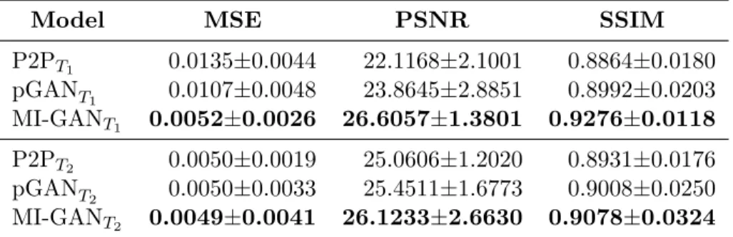
Table 3.1: Comparison between P2P, pGAN and MI-GAN. Values in boldface represent best performance values. Reported values are mean± std.

Model MSE PSNR SSIM

P2PT1 0.0135±0.0044 22.1168±2.1001 0.8864±0.0180 pGAN_T 1 0.0107±0.0048 23.8645±2.8851 0.8992±0.0203 MI-GAN_T1 0.0052±0.0026 26.6057±1.3801 0.9276±0.0118 P2PT2 0.0050±0.0019 25.0606±1.2020 0.8931±0.0176 pGAN_T 2 0.0050±0.0033 25.4511±1.6773 0.9008±0.0250 MI-GAN_T2 0.0049±0.0041 26.1233±2.6630 0.9078±0.0324

Ground Truth

1 P2P 1 pGAN1 MI-GAN 1 Ground Truth

2 P2P2 pGAN2 MI-GAN2

ℎ

Figure 3.1: Qualitative results for P2P, pGAN, and MI-GAN. Left subfigure (columns (a) through (d)) visualize the performance of three models in synthesis ofT1 sequence. The second subfigure (columns (e) through (h)) show synthesizedT2 sequences for each of the

Table 3.1 presents MSE, PSNR and SSIM results for all three model architectures and their variants. We observe that both variants of MI-GAN outperform both P2P and pGAN models in all metrics.

Comparing MI-GAN_T1 and the baseline P2P_T1, MI-GAN_T1 outperformed by 61.48% in terms of MSE (p < 0.05), 20.29% in PSNR (p < 0.05) and 4.64% in SSIM (p < 0.05). MI-GAN_T1 also outperformed the state-of-art single-input single-output model pGAN_T

1, in all metrics, with improvements of 51.40% in MSE (p < 0.01), 11.48% in PSNR (p < 0.05) and 3.15% in SSIM (p <0.05).

Similarly for T2 synthesis, MI-GANT2 outperforms both P2PT2, pGANT2. With respect to P2P_T2, MI-GAN_T2 performs better by 2% in MSE, 4.24% in PSNR and 1.64% in terms of SSIM. Compared to pGAN_T2, MI-GANT2 shows improvement of 2% in MSE, 2.64% in PSNR and 0.77% in SSIM. Although the quantitative improvement in T2 synthesis was modest

compared to both P2P_T2 and pGAN_T

2, we notice interesting qualitative improvements, visible in Figure 3.1, where MI-GANT2 managed to synthesize the pathology region which other methods failed to generate.

These improvements of MI-GAN over P2P and pGAN models can be attributed to the availability of multiple sequences as input, which the network utilizes to synthesize missing sequences. The qualitative results showing axial slices from a test patient are provided in Figure 3.1 in which red arrow points to the successful synthesis of tumor regions in the case of MI-GAN, which was possible due to tumor specific information present in the available three sequences about the various tumor sub-regions (edema, enhancing and necrotic core) in the input sequences, which is not available in its entirety to the single-input single-output methods. We also notice that MI-GAN performs consistently for a single patient, without showing significant deviation from the ground truth intensity distributions in bothT1 and

T2.

Superior quantitative and qualitative results showing MI-GAN outperforming P2P and pGAN reinforce the hypothesis that using multiple input sequences for the synthesis of a missing sequence is objectively better than using just one input sequence. Moreover, using multi-input methods reduces the number of required models by an order of magnitude, where for a multi-input single-output (many-to-one) only 4 models would be required, compared to 12 for single-input single-output (one-to-one) model (C(C −1) when C = number of sequences = 4). A multi-input multi-output (many-to-many) model which we explore in this work, improves this further by just requiring a single model to perform all possible synthesis tasks for a given C, leading to enormous computational savings during training time.

3.2

T

Synthesis (MISO)

In this second set of experiments we train our MM-GAN model to synthesizeT2f lairsequence

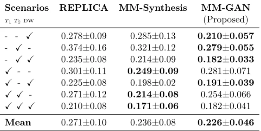
in the presence of a varied number of input sequences (one, two or three). Contrasting from the MI-GAN models, this model is trained to generalize on number of different scenarios depending on the available input sequences. In this case, the number of valid scenarios are 7. We perform validation on the ISLES2015 dataset in order to directly compare with REPLICA [22] and MM-Synthesis [5]. The quantitative results are given in Table 3.2. We note that the proposed MM-GAN (0.226±0.046) clearly outperforms REPLICA’s unimodal synthesis models (0.271±0.10) in all scenarios, as well as MM-Synthesis (0.236±0.08) in majority (4/7) scenarios. Our method also demonstrates an overall lower MSE standard deviation throughout testing (ranging between [0.03, 0.07], compared to REPLICA [0.08, 0.16] and MM-Synthesis [0.02, 0.13]) in all scenarios but one (T2 missing). The qualitative results for ISLES2015 are shown in Figure 3.2. Compared to MM-Synthesis (from qualita-tive results shown in their original paper [5]), our results are objecqualita-tively sharper, with lower blurring artifacts. MM-GAN also preserves high frequency details of the synthesized se-quence, while MM-Synthesis and REPLICA seem to miss most of these details. We request the readers to refer to the original MM-Synthesis [28] manuscript’s Figures 5 and 6 for com-parison with our proposed MM-GAN’s qualitative results given in Figure 3.3 of the current manuscript. Qualitatively from Figure 3.2, MM-GAN follows the intensity distribution of the realT2f lair sequence in its synthesized version ofT2f lair.

Table 3.2: Comparison with unimodal method REPLICA and multimodal method MM-Synthesis. The reported values are mean squared error (MSE). Boldface values represent lowest values of the three methods for a particular scenario.

Scenarios REPLICA MM-Synthesis MM-GAN

T1T2DW (Proposed) - - _X 0.278±0.09 0.285±0.13 0.210±0.057 - _X - 0.374±0.16 0.321±0.12 0.279±0.055 - _{X X} 0.235±0.08 0.214±0.09 0.182±0.033 X - - 0.301±0.11 0.249±0.09 0.281±0.071 X - _X 0.225±0.08 0.198±0.02 0.191±0.039 X X - 0.271±0.12 0.214±0.08 0.254±0.066 X X X 0.210±0.08 0.171±0.06 0.182±0.041 Mean 0.271±0.10 0.236±0.08 0.226±0.046

We found that using CL based learning did not help in MISO experiments, as the pres-ence of more sequpres-ences does not necessarily increase the amount of information available. For example, the presence of bothT1andT2does not result in betterT2f lairsynthesis (MSE

0.2541) compared to the presence of DW alone (MSE 0.2109). This is because, for every missing sequence, there tends to be some “highly informative” sequences that, if absent,

1110 1100 1010

0110 1000 0100 0010

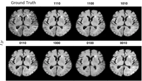
Figure 3.2: Qualitative results from T2f lair synthesis experiments with ISLES2015 dataset.

The order of scenario bit-string isT1,T2, DW, T2f lair , where a zero (0) represents missing

sequence, while a one (1) represents an available sequence. We note that the presence of multiple sequences (scenario 1110) qualitatively matches the closest to the ground truth, with sharp boundaries between white and grey matter, as well as less blurring artifacts compared to scenarios with two or just one available sequences. Patient images shown here are from VSD ID 70668 from ISLES2015 SISS cohort.

reduces the synthesis performance by a larger margin. On the other hand, the presence of these highly informative sequences can dramatically boost performance, even in cases where no other sequence is present. Due to this, the assumption that leveraging a higher number of present sequences implies an easier case (i.e. more accurate synthesis) does not hold, and thus it becomes problematic to rank scenarios based on how easy they are, which renders CL useless in this case. Globally (for all valid scenarios, presented in next subsec-tion), however, this assumption tends to hold due to the complex nature of interactions between sequences. CL helps tremendously in achieving a stable training of the network in the subsequent experiments (MIMO). For MISO, every scenario was shown to the network with uniform probability, throughout training.

3.3

Validation of Key Components

3.3.1 Imputation Value and Curriculum Learning

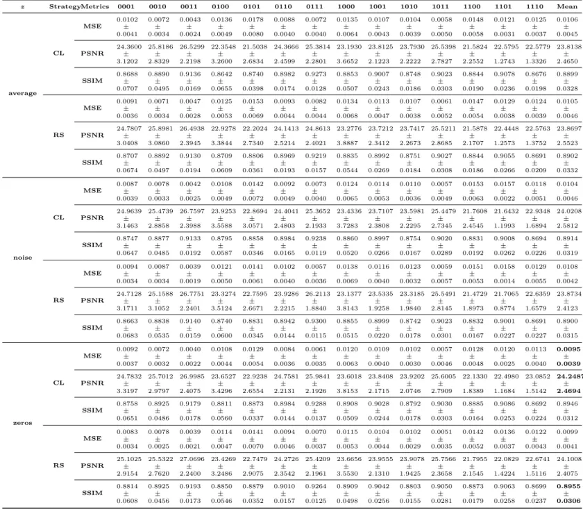
In our proposed multi-input multi-output MM-GAN model, the missing sequences during both training and test time has to be imputed with some value. In order to identify the best approach for imputing missing slices, we test MM-GAN with three imputation strategies, wherez= average of available sequences, z= noise, andz= zeros.

We also test curriculum learning (CL) based training strategy where the network is initially shown easier examples followed by increasingly difficult examples as the training

progresses. We compare this approach with random sampling (RS) method, where scenarios are uniformly sampled during training regardless of the number of missing sequences. In order to test the effectiveness of CL based learning, we report results with CL-based learning as well as random sampling (RS) based learning for each imputation strategy.

The results for our experiments are given in Table 3.3. The imputation valuez= zeros performed the best when CL based training strategy is adopted (MSE 0.0095 and PSNR 24.2487), and was slightly outperformed in SSIM by z = zeros with RS sampling (SSIM 0.8955). z = noise performs slightly worse than zero imputation, but better than the z = average imputation for both CL and RS strategies. This may be due to the fact that imputing with a fixed value (zero vs noise/average) provides network with a clear indication about a missing sequence (implicit conditioning), as well as relieves it from learning weights that have to generalize for variable values imputed at test time. Imputing with zeros also removes the non-deterministic behaviour that was prevalent inz= noise, where each test run would yield slightly different quantitative (though mostly similar qualitative) results. For our final benchmark results on LGG and HGG cohorts in BraTS2018, we set z= zeros and use CL based learning strategy to train the networks.