ICES WKADSAM REPORT 2010

(1)

SCICOM

S

TEERING

G

ROUP ON

S

USTAINABLE

U

SE OF

E

COSYSTEMS

ICES

CM

2010/SSGSUE:10

R

EF

.

SCICOM,

ACOM

Report of the Workshop on Reviews of Recent

Advances in Stock Assessment Models

World-wide: "Around the World in AD Models"

(WKADSAM)

27 September - 1 October 2010

Nantes, France

(2)

International Council for the Exploration of the Sea

Conseil International pour l’Exploration de la Mer

H. C. Andersens Boulevard 44–46 DK-1553 Copenhagen V Denmark Telephone (+45) 33 38 67 00 Telefax (+45) 33 93 42 15 www.ices.dk [email protected]

Recommended format for purposes of citation:

ICES. 2010. Report of the Workshop on Reviews of Recent Advances in Stock As-sessment Models Worldwide: "Around the World in AD Models" (WKADSAM), 27 September - 1 October 2010, Nantes, France. ICES CM 2010/SSGSUE:10. 122 pp. For permission to reproduce material from this publication, please apply to the Gen-eral Secretary.

The document is a report of an Expert Group under the auspices of the International Council for the Exploration of the Sea and does not necessarily represent the views of the Council.

(3)

Executive summary

The Workshop on the Reviews of Recent Advances in Stock Assessment Models Worldwide “Around the World in AD Models” (WKADSAM) was convened in Nantes, France during autumn 2010 as the first meeting of the three-year ICES Strate-gic Initiative on Stock Assessment Methods (SISAM). Despite prevailing economic difficulties which have affected travel budgets for many institutes, the Workshop was successful in attracting participants from all over the world: 21 of the 32 attendees came from outside Europe.

The main interest for the Workshop lay in having a group of practicing stock assess-ment scientists and model developers discuss the models that are currently used around the world. The goal during the Workshop was to compare and contrast dif-ferent modelling approaches in a systematic manner to provide guidance to ICES working groups on when particular models or approaches would be or would not be useful. The Workshop was specifically not a competition. In preparation for the meet-ing, a catalogue of models was prepared through the ICES Working Group on Meth-ods of Stock Assessment (WGMG) as a starting point for discussions and included as an annex to this report. Because, the catalogue alone is not enough for colleagues to understand fully the practical details of a particular model, the presentation of case studies focussing on which problem each method has fixed was particularly impor-tant for helping to guide stock assessment scientists to a limited number of possible models to consider. Any conclusions were not to be prescriptive, but rather to present information clearly and fairly to allow informed model selection.

The first three days of the Workshop were taken up with presentations and discus-sions of methods and approaches. Much of the remaining two days was occupied with discussions about the hands-on experience of WKADSAM participants of the model packages presented, the important issue of model selection, the development of agreed terminology, and the generation of general conclusions from the meeting, along with recommendations for the forthcoming 2012 Conference. The general con-clusions in brief are:

• WKADSAM recognizes the importance of the distinction that ICES has made between benchmark and update stock assessments. During the benchmark process for a given stock, a number of candidate research models should be applied to demonstrate the robustness of the advisory model. The advisory model (used for update assessments) should not be reviewed as part of the update advice process: the update assessments should only be subject to a technical audit. The purpose of the advisory model is not to understand every underlying real-world process but to provide robust ad-vice.

• The order of importance for stocks for consideration in benchmark assess-ments should be: 1) stocks that are currently assessed incorrectly; 2) stocks that are not currently assessed and for which an assessment is required; 3) stocks for which the assessment could potentially be improved.

• The development of new stock assessment approaches should focus on situations where standard models cannot be applied, due to data or proc-ess constraints.

• New members of ICES assessment WGs (who have assessment responsi-bility) are encouraged to be able to write a simple stock assessment model as a minimum.

(6)

• WKADSAM does not recommend the use of one standard model package for ICES assessments, nor should all assessments use different methods. Selection of both the modelling approach and software package to be used for each stock should be based on a thoughtful consideration of the avail-able data, biology of the stock, management requirements, statistical prin-ciples, and (importantly) available expertise.

(7)

1 Introduction

1.1 Terms of Reference (ToRs)

The ICES Workshop on Reviews of Recent Advances in Stock Assessment Models Worldwide “Around the World in AD Models” (WKADSAM) chaired by Coby Needle, UK*, and Chris Legault*, USA will meet in Nantes, France, 27 September to 1 October 2010 to, collate, review and comment on stock assessment methods currently in use around the world.

This will be part of the ICES initiative on stock assessments methods. The workshop was to:

a ) Determine the key techniques and approaches used to assess fish stocks b ) Consider inter alia utility, ease of use, estimation procedures, robustness,

suitability to different data richness, applicability to data poor situations, and relevance of assumptions in the models

c ) Summarize the advantages and disadvantages of the various methods, and describe the appropriate use.

d ) Comment on demonstrations by model developers of the utility of meth-ods with case studies and simulated datasets, focussing on the question: What problem has the method fixed?

e ) Prepare the groundwork for a following workshop in 2011 or 2012 (see ini-tiative plan below)

WKADSAM formed the first phase be part of the ICES Strategic Initiative on Stock Assessment Methods (SISAM). WKADSAM reported by January 2011 for the atten-tion of the SISAM Steering Group.

1.2 Intended approach

In preparation for the meeting, it became clear that the ToRs were causing a degree of confusion among potential participants as to what exactly was to be achieved by the Workshop. To address this, the Chairs circulated a note which was intended to clarify the issues. This had implications for the outcomes of the meeting, and it is germane to summarize this note here, as follows.

This workshop was not to be a “Methods Olympics” where competing models battle for designation as the “best” model. There simply would not have been sufficient time during a week-long meeting to apply a large number of models to the large number of datasets that would be needed to ensure “fairness” (in a competitive sense). Such a competition would result in models that correspond most closely to the data and processes performing best, but the ability to generalize the results to all ICES assessments would be quite limited. The e-mail discussions preceding the Workshop served to demonstrate how difficult it is to set up such comparative tests appropriately.

Instead, the main interest lay in having a group of practicing stock assessment scien-tists and model developers discuss the models that are currently used around the world. A necessary first step for this discussion was to catalogue the currently avail-able models, which the ICES Working Group on Methods of Fish Stock Assessment (WGMG) is currently undertaking. The goal during the workshop was to use this catalogue as a starting point for discussions. The catalogue alone is not enough for

(8)

colleagues to understand fully the practical details of a particular model, and uncov-ering these was always likely to fill a considerable part of the available time.

Although ToR c) may have misled people to think this meeting would be a model competition, the Chairs viewed it instead as a way to help ICES assessment working groups sort through the many available models outside those currently used for their particular assessment to find potential alternatives. The presentation of case studies showing what problem each method has fixed (ToR d) was particularly important for helping to guide stock assessment scientists to a limited number of possible models to consider. Any conclusions were not to be prescriptive, but rather present information clearly and fairly to allow informed model selection.

1.3 Terminology

Towards the end of the meeting, concerns were expressed by several participants that terms such as “model” and “software package” were being used interchangeably, and in a way that could confuse subsequent readers of the report. To address this, two definitions were made that will be used throughout:

• Modelling approach: set of equations and data that allow estimation of population abundance or other metrics of interest

• e.g. statistical catch-at-age, virtual population analysis, time-series analysis

• Software package: a specific case of a modelling approach that is named • e.g. Stock Synthesis, CASAL, Multifan-CL, SAM, etc.

There was also considerable discussion over classifications of software-package fami-lies. WKADSAM settled on the following genre set:

• Flexible, multipurpose: packages which are intended to be applicable to a broad range of stock and data situations. Examples from the WKADSAM meeting include SS3, CASAL and Multifan-CL.

• Specific, data issue-driven: packages which can be applied to a number of stocks, but which are specific in their data requirements. Examples from the WKADSAM meeting include XSA, Adapt VPA, and many of the pack-ages currently used by stock assessment WGs.

• Custom, stock specific: bespoke code which is written for a particular purpose and is not intended to be widely used.

The advantages and disadvantages of each of these families are discussed further throughout this report, and in particular in the Conclusions (Section 4).

1.4 Report structure

The bulk of this report is taken up by considerations of the software packages pre-sented at the WKADSAM meeting (Section 2), which is intended to cover most of ToRs a) – d). Each subsection of Section 2 contains the extended summary of the model package presented (prepared by the presenter), along with a summary of the discussion following each presentation as collated by the relevant rapporteur. Several subsections also include a summary of the presentation itself from the rapporteur. It should be noted that the material provided by the presenter of each model or package has been included in the report without any editing for content – there-fore, some of the conclusions reached in these sections may not necessarily repre-sent a consensus view.

(9)

Section 3 summarizes the hands-on experience of WKADSAM participants of the model packages presented, and concludes that such experience is actually quite lim-ited. It also covers an important case study for the issue of model selection, looking into the decisions taken during the recent benchmarking process for ICES hake stocks. Section 4 then offers general conclusions from the meeting, along with rec-ommendations for the forthcoming 2012 Conference.

Finally, the available software package descriptions that have been collated by the ICES Working Group on Methods of Fish Stock Assessment (WGMG) during 2010 are brought together in a series of annexes. Not all of these packages were discussed during the WKADSAM meeting, but it is worthwhile to bring all the descriptions together in one place for future reference.

2 Software packages and themes

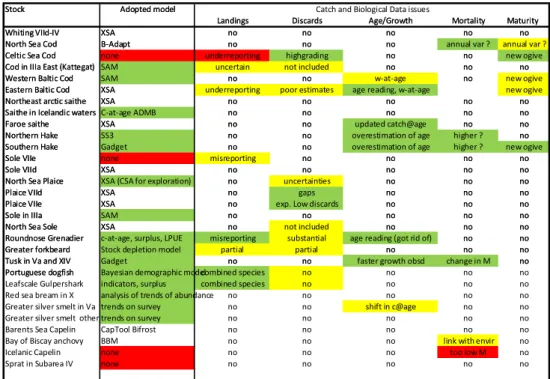
The following table summarizes the software package (or theme) presentations given at WKADSAM. For each of the packages, a description template was also filled in: these can be found in Annex 2, along with description templates for a number of packages in use in ICES and elsewhere that were not presented at WKADSAM.

SECTION SOFTWARE PACKAGE /THEME PRESENTER

2.1 SAM Anders Nielsen

2.2 BREM Verena Trenkel

2.3 Stock Synthesis 3 Rick Methot

2.4 MULTIFAN-CL Shelton Harley

2.5 CASAL Matt Dunn

2.6 TINSS Steve Mattell

2.7 CSA Benoit Mesnil

2.8 Adapt VPA Chris Legault

2.9 ASAP Chris Legault

2.10 SURBA Coby Needle

2.11 XSA Chris Darby

2.12 B-ADAPT Chris Darby

2.12 General issues in

benchmarks

Lionel Pawlowski

2.13 Generic model features Doug Butterworth

2.1 SAM

2.1.1 Description

The state-space fish stock assessment model (SAM) was summarized to the group with focus on the rationale behind using random effects to describe the underlying random variables that are not observed (fishing mortalities and stock sizes). SAM is an age structured time-series model designed to be an alternative to the (semi-) de-terministic procedures (e.g. VPA, Adapt, and XSA) and the fully parametric statistical catch at-age models (e.g. SCAA, and SMS). Compared to the deterministic proce-dures it solves the problem of falsely assuming catches-at-age are known without errors, and in addition the problem of selecting appropriate so-called ‘shrinkage’ and in certain cases convergence problems in the final years. Compared to fully paramet-ric statistical catch at-age models SAM avoids the problem of fishing mortality being restricted to a parametric structure (e.g. multiplicative), and many problems related

(10)

to having too many model parameters compared to the number of observations (e.g. borderline identification problems, convergence issues, and asymptotic results). In addition the model has a number of appealing properties. It allows selectivity to gradually evolve during the data period, it allows missing data, and finally it esti-mates the underlying process noise, which is useful for forward predictions.

Previous implementations of state-space assessment models (Gudmundsson 1987, 1994, and Fryer 2001) have been based on the extended Kalman filter, which uses a first order Taylor approximation of the non-linear parts of the model. The current implementation is based on the Laplace approximation which is better suited to han-dle non-linearities, and further validated by importance sampling.

It was presented how the recent decision to change XSA-shrinkage from 0.5 to 0.75 for Eastern Baltic Cod radically changed the perception of the stock in the final year to be more in line with the state space assessment model. The presenter argued against using ad-hoc criteria for setting these shrinkage parameters.

The state-space model has previously been validated at the methods working group by comparing to existing assessments and via simulated data. To further validate the model, it was extended to allow jumps in the underlying process to follow a mixture between a Gaussian and a fat-tailed Cauchy distribution, as opposed to a purely Gaussian. The model applied to North Sea Cod estimated the Cauchy fraction to be zero, and even forcing the Cauchy fraction to be 30% did not make the underlying process take noticeable sharper jumps. Finally a recent extension to allow the fishing mortality processes to be correlated was presented.

SAM is currently run for the following stocks in ICES: Kattegat Cod, Western Baltic Cod, Sole in 3A, Eastern Baltic Cod, North Sea Sole, Plaice in 3A, and North Sea Cod. Of these the state-space assessment model is primary for the first three stocks, and included as exploratory for the remaining. In addition to the stocks mentioned above it has been applied to other stocks (Western Baltic spring-spawning herring, North Sea Haddock, 3PS Cod, and Georges Bank Yellowtail Flounder) for testing purposes, and has performed well.

A simple web interface (http://www.stockassessment.org) to the state-space assess-ment model was presented. Collaboration at assessassess-ment working groups are often reduced to one or two members doing the actual assessment modelling, and remain-ing workremain-ing group members reviewremain-ing and commentatremain-ing on the results only. Part of the reason most working group members don’t even try to reproduce the assess-ment, is that it takes a lot of work to get everything set up correctly. Typically several programs (specific versions) need to interact and the data need to be on a specific format. The web interface presented completely removes this obstacle. Once the stock coordinator has set up an assessment all members can reproduce the assessment and all the resulting graphs and tables simply by logging in and pressing ‘run’. The work-ing group members can also experiment with the model configuration and input data and easily compare the results. It would clearly be beneficial to have more hands and eyes on the details of each assessment.

Rapporteur’s summary of presentation

SAM is an age-structured state-space model, with stochastic recruitment coming in every year (assuming some stock–recruitment relationship and lognormally distrib-uted recruitment deviations). Log-normal process errors are assumed along cohorts. Fishing mortality follows a random walk in log-space with normally distributed

(11)

in-crements, applying, in principle, an independent random walk for each age. The data consist of catch numbers-at-age and survey indices-at-age, with observation error considered both in the catch and the survey indices. Model parameters consist of the variances of the process and observation errors, including the variance of the random walk for the log(fishing mortality-at-age) , the surveys’ catchabilities and the parame-ters intervening in the stock–recruitment relationship. SAM is implemented in AD Model Builder, using its random effects module. A web interface has been developed for SAM, in order to facilitate its use. The model is used for several ICES stocks, ei-ther as the main assessment or as an alternative exploratory assessment. In order to allow for some potentially big jumps in F values in some time periods, the normal distribution for the log(F) increments can be replaced by a mixture of a normal and a t-distribution with low degrees of freedom. Another alternative explored for model-ling log(F) is to have the normal increments correlated, instead of independent, across ages. Perfect correlation between the ages would correspond to separable fish-ing mortality, but with the annual factor of the fishfish-ing mortality followfish-ing a random walk (in log-space) rather than being treated as a separate parameter for each year. Development of SAM continues and new features will be added.

2.1.2 Summary of WKADSAM discussion

The presentation was well received and the model was found to be useful and prom-ising.

A remark was made about the difficulties (or near impossibility) often encountered when trying to estimate both process and observation error in state-space models. It is often found that the estimate of one of the variances goes to zero and, for example, fixing the ratio of both variances has sometimes been used as a “fix”. The author said that the problem had not been encountered in the applications that have used SAM to date. A SAM like method was experimented with for sandeel, a species with short cohorts and very noisy data, and for that it was impossible to split observation and process error.

The question of whether a comparison had been performed between SAM and mod-els where F is treated as a parameter, even if assigned a random walk distribution, was asked. The answer was negative. The importance of estimating the model pa-rameters instead of using arbitrary values was highlighted.

Pros and cons of running the program directly on a web server were discussed. In particular, some people felt that this could be inconvenient as it required having Internet access. The author explained that all relevant files could be downloaded to one’s own PC and run locally. He felt that having the web setting made things more clear and transparent and that the web interface could make things easier for non-experienced users.

The improved ability of the model to detect jumps in F by using a mixture of a nor-mal and a t-distribution with low degrees of freedom was discussed. Some questions were raised about the ability of the model to detect such changes if these were of smaller magnitude than the ones in the example considered.

The author highlighted the fact that model fitting follows a clearly defined statistical procedure (maximum likelihood), hence avoiding difficult decisions like choosing an appropriate level of shrinkage in XSA.

Presently SAM does not allow inputting catches at the fleet level, only at stock level. It allows tuning fleets, but they are currently treated as surveys.

(12)

Work is going on at present to develop a multistock configuration of SAM.

SAM is a purely age-structured model. No length-structured configuration has been developed.

Robustness to poor ageing has not been examined and ageing errors are not explicitly modelled in SAM, but observation noise on age-classified catches is part of the model.

2.2 BREM (Two-stage Biomass Random Effects Model)

2.2.1 Description: Application of BREM to Bay of Biscay anchovy

The text provided by the presenter for this Section outlines the results of a case study. Details on the method itself can be found in the relevant table in Annex 2.

2.2.1.1 Data and model

Two time-series of biomass estimates for age 1 and total biomass were available for anchovy in the Bay of Biscay. The first one is obtained using the daily egg production method, referred to as DEPM series, and the second on using acoustics and identifica-tion trawl hauls, the acoustic series.

To make the model identifiable, one of the catchability parameters has to be fixed. Two choices are explored: 1) qbac°ustic =1; 2) qbDEPM = 1. Note that the recruit and total

survey indices per method are assumed to have the same CV. 2.2.1.2 Results

Preliminary analyses

To check the consistency of the survey indices, a cohort plot of acoustic biomass indi-ces-at-age was produced (Figure 1 left). The plot shows that successive indices of cohorts decreased as expected with the exception of the 2005 cohort for which the biomass index for age 1 was substantially smaller than for age 2 one year later (high-lighted by a circle in figure 1). Indeed, survey indices for both the acoustics and the DEPM were unusually low for age 1 and also total biomass in 2005 (Figure 1 right). Thus it seems possible that the 2005 survey indices, at least for age 1, do not reflect stock biomass in the same manner as in other years. Given that the model assumes constant catchabilities across years, this would violate the assumptions of the model. Therefore an additional model fit was carried out where all data for 2005 was re-moved.

(13)

1.0 1.5 2.0 2.5 3.0 3.5 4.0 0 1000 2000 3000 4000 5000 Cohorts Age A c ous ti c bi om as s i ndex 2000 2001 2002 2003 2004 2005 2006 2007 2008 1990 1995 2000 2005 0 20 40 60 80

Age 1 biomass ind

DEPM acoustics 1990 1995 2000 2005 20 40 60 80 100

Total biomass ind

de

Figure 1. Cohort plot for acoustic biomass indices (left) and time-series of all survey indices (right).

Brem assumes that recruitment follows a lognormal distribution with no correlation between subsequent years. To check the validity of this assumption, the autocorrela-tion in survey indices for age 1 was calculated for the years 2000–2009 (Figure 2). Due to missing values it could not be calculated for earlier years. The results indicate that there was no autocorrelation in neither the acoustics nor the DEPM survey series.

0 2 4 6 8 -0. 5 0. 0 0. 5 1. 0 C Acoustics age 1 in 0 2 4 6 8 -0. 5 0. 0 0. 5 1. 0

DEPM age 1 index

Figure 2. Autocorrelation analysis of biomass indices for age 1 for the period 2000–2009 (right).

Model fits

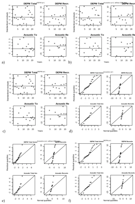
Standardised residuals were plotted against years to check patterns in residuals (Fig-ure 3a-c). No obvious patterns occurred apart from an autocorrelation of standard-ized residuals in the final 5–8 years for total biomass estimates; in particular for the DEPM survey indices. Quantile-quantile plots (Figure 3d-f) showed that residuals for total biomass indices were approximately lognormally distributed as assumed in the model while residuals for recruit biomass did not follow the assumed lognormal distribution as they do not lie on the diagonal line as expected.

(14)

a) 5 10 15 20 -2 -1 0 1 2 3 DEPM Total 5 10 15 20 -10 -5 0 5 10 DEPM Recru 5 10 15 20 -2 0 1 2 3 Acoustic Tot 5 10 15 20 -15 -5 0 5 10 Acoustic Re DEPM q=1 Years S tandar di s ed r es idual s b) 5 10 15 20 -2 -1 0 1 2 3 DEPM Total 5 10 15 20 -5 0 5 10 DEPM Recru 5 10 15 20 -2 0 1 2 3 Acoustic Tot 5 10 15 20 -6 -2 2 4 6 Acoustic Re

Acoustics q=1; without 2005 data

Years S tandar di s ed r es idual s c) 5 10 15 20 -2 -1 0 1 2 3 DEPM Total 5 10 15 20 -10 -5 0 5 10 DEPM Recru 5 10 15 20 -2 0 1 2 3 Acoustic Tot 5 10 15 20 -15 -5 0 5 10 Acoustic Re DEPM q=1 Years S tandar di s ed r es idual s d) -2 -1 0 1 2 3 -2 -1 0 1 2

3 DEPM Total bioma

-10 -5 0 5 10 -10 -5 0 5 10 DEPM Recruits -2 -1 0 1 2 3 -2 0 1 2 3

Acoustic Total biom

-15 -5 0 5 10 -15 -5 0 5 10 Acoustic Recruits Acoustics q=1 Normal quantiles R es idual quant il es e) -2 0 2 4 6 -2 0 2 4 6

DEPM Total bioma

-5 0 5 10 -5 0 5 10 DEPM Recruits -2 0 2 4 6 -2 0 2 4 6

-5 0 5 10 -5 0 5 10 Acoustic Recruits Acoustics q=1; without 2005 data

Normal quantiles R es idual quant il es f) -2 -1 0 1 2 3 -2 -1 0 1 2

3 DEPM Total bioma

-10 -5 0 5 10 -10 -5 0 5 10 DEPM Recruits -2 -1 0 1 2 3 -2 0 1 2 3

-15 -5 0 5 10 -15 -5 0 5 10 Acoustic Recruits DEPM q=1 Normal quantiles R es idual quant il es

Figure 3. Residual plots. Standardised residuals and quantile-quantile plots by survey series. a) & d) qbac°ustic=1; b) & e) qbac°ustic=1, without 2005 data; c) & f) qbDEPM=1.

Relative stock estimates

The Brem model provides relative stock estimates whose absolute level is condi-tioned by the assumptions made for survey catchability. Setting qbac°ustic=1 led to

sys-tematically higher biomass estimates (black continuous line in Figure 3) compared to the case than qbDEPMc=1 (red dashed line in Figure 4). However, relative time-trends

were similar. Removing data for 2005 (qbac°ustic=1) affected all estimates for the years

2005–2009 (green dotted line in Figure 4). In particular, recruit estimates were in-creased and total biomass estimates somewhat dein-creased in recent years. Total bio-mass estimates including CVs are provided in table 1. Setting qbac°ustic=1 and including

data for the year 2005 provided generally the most precise (smallest CV) biomass estimates, though not for the final years.

(15)

1990 1995 2000 2005 0 50 100 15 Year R ec rui tm ent bi om a Acoustics qb=1 DEPM qb=1 Acoustics qb=1, without 2005 1990 1995 2000 2005 0 50 100 15 Year T ot al bi om as s Acoustics qb=1DEPM qb=1 Acoustics qb=1, without 2005

Figure 4. Model estimates for anchovy recruit biomass (age 1) and total biomass in the Bay of Biscay using acoustic and DEPM biomass indices. The black and red lines refer to models with different hypothesis on survey catchability. The green line was obtained when data for 2005 was removed.

Table 1. Relative total biomass estimates using Brem model and two survey time-series.

QBACOUSTIC=1 QBACOUSTIC=1& WITHOUT 2005 DATA QBDEPMC=1

Year Total biomass CV Total Biomass CV Total Biomass CV

1987 59.26 0.28 58.62 0.33 44.30 0.26 1988 85.73 0.28 82.91 0.44 61.08 0.27 1989 26.56 0.53 30.88 0.77 18.89 0.53 1990 128.41 0.27 119.04 0.44 91.19 0.26 1991 46.51 0.46 51.35 0.66 33.03 0.46 1992 113.51 0.25 114.04 0.38 80.61 0.24 1993 55.75 0.70 63.32 0.77 39.59 0.70 1994 57.55 0.41 57.99 0.63 40.87 0.40 1995 74.75 0.32 75.00 0.49 53.08 0.31 1996 58.05 0.43 58.71 0.59 41.22 0.42 1997 65.09 0.32 66.94 0.47 46.22 0.31 1998 102.61 0.37 97.41 0.50 72.87 0.36

(16)

QBACOUSTIC=1 QBACOUSTIC=1& WITHOUT 2005 DATA QBDEPMC=1 1999 88.65 0.45 83.16 0.63 62.96 0.44 2000 102.99 0.29 105.34 0.35 73.14 0.29 2001 118.12 0.32 118.05 0.46 83.89 0.32 2002 75.99 0.48 76.40 0.64 53.96 0.48 2003 39.12 0.66 39.65 0.75 27.78 0.65 2004 39.08 0.45 41.72 0.45 27.75 0.45 2005 14.61 1.11 48.45 0.68 10.37 1.10 2006 29.97 0.43 34.74 0.56 21.29 0.43 2007 42.21 0.46 41.55 0.39 29.97 0.46 2008 33.88 0.93 27.63 0.58 24.06 0.92 2009 33.44 1.06 27.98 0.53 23.75 1.05

2.2.1.3 Summary of WKADSAM discussion

Recruitment (age 1) biomass is modelled separately to total biomass (which includes recruitment) in order to make full use of recruitment information which for the chovy application comes from acoustic and DEPM survey estimates. For Biscay an-chovy, the population dynamics is driven by recruitment, with a comparatively small amount of the population subsequently contributing to the total biomass, hence why it is useful to model recruitment in addition to total biomass.

The model as applied to Biscay anchovy has potentially 4 estimates of catchability q (one each for the survey type – acoustic and DEPM – and one each for the stage – recruitment and total biomass), but the recruitment and total biomass q are estimated separately. This gives four q estimable parameters, but 1 is needed to be fixed (to 1) while the others are estimated. Which of these is fixed does matter because the two sets of time-series (acoustic vs. DEPM) have missing data in different places.

It may have been useful to include catch data for the period for which it was still re-garded as reliable (if there was such a period), as this would have helped with the scaling, but this model was developed in the context of producing survey-only meth-odology, so it was not appropriate to include catch data in this case.

The two time-series for recruitment (age 1) biomass (acoustic and DEPM) showed good agreement (although there were also differences) – it was pointed out that the age 1 estimates for the two surveys were not entirely independent as the age struc-ture from the acoustic estimates were used to partition the DEPM estimates after the surveys were completed. There was no exchange of information between the surveys for the total biomass.

Concerns were raised about the 2005 estimates because of inconsistency in q (fish might have been close in-shore that year so may have been missed). An exploratory run excluded 2005 entirely from the analysis, and resulted in changed estimates for 2005 and a re-scaling of the total biomass trajectory. However, omitting 2005 may imply that, given that recruitment is modelled as a random effect based on a log-normal distribution, the model will simply replace the 2005 data with the mean of the assumed distribution. Questions were raised about whether this was more justifiable than using the actual data.

Estimates of population trends from BREM showed more variation than the SAM model (a state-space model, which also uses the random effects concept), but this is because recruitment is very variable for Biscay anchovy, resulting in the random

(17)

walk process for biomass growth contributing less to the overall dynamics. However, the SAM model does not always produce smooth population trends – this depends on the underlying data.

An analysis of the q-q plot for the random effects in recruitment showed that the lognormal assumption for recruitment was not ideal. Estimating recruitment values each year as an alternative to modelling random effects was not tried. There was a problem with estimation the variance for the g random effect because of the highly variable recruitment (which is the other random effect). For Biscay anchovy, the two variances associated with recruitment and biomass growth were not easily identifi-able; although the variance for recruitment could be always estimated, it could not always for biomass growth. This is probably indicating that the model is close to not being identifiable.

Problems with assuming a lognormal distribution for recruitment where highlighted. Essentially, the problem is one of asymmetry because strong year classes have a lot of information about their strength, but weak year classes are lost in the noise. Estimates of recruitment have distributions with thinner lower tail than the actual recruitment, so that the really weak year classes are not estimated to be as weak as they should be. In contrast, estimating the strength of strong year classes does not pose the same problem.

Given that for BREM, catch is excluded, and recruitment is not dependent on bio-mass, this must pose difficulties for communicating results to managers. Neverthe-less, the survey does contain information about recruitment and impact of fishing. The ease of use of the BREM model depends on the user’s knowledge of ADMB code, because there is no front-end available. The available code could be used as a starting point for adapting the approach to a particular situation and data. However, there is the problem that ICES WGs do not necessarily contain the sort of people that can do this.

As with any model, the application to a new stock will always need an expert over-view of what is done initially. This requirement can be relaxed once the method is ready for repeated use.

2.3 Stock Synthesis 3 (version 3.11b)

Stock Synthesis (SS) provides a statistical framework for calibration of a population dynamics model using a diversity of fishery and survey data. The following refers to version 3.11b, dated September 2010.

2.3.1 Description

Language

SS currently is compiled using ADMB version 7.0.1 using the Microsoft C++ compiler version 6.0.

Programmer / Contact Person

Dr Richard D. Methot, Jr., NOAA Fisheries – Office of Science and Technology, Northwest Fisheries Science Center, 2725 Montlake Boulevard East, Seattle, WA 98112. e-mails: [email protected]

(18)

Distribution Limitation

The model and a graphical user interface are available from the NOAA Fisheries Stock Assessment Toolbox website: http://nft.nefsc.noaa.gov/. Only executable code is

routinely distributed, along with manual and sample files. However, under certain circumstances, source code may be obtained from the author upon request and with agreement to certain restrictions.

Compiler Needs / Stand-Alone

SS runs as a DOS program with text-based input or can be invoked from a graphical interface (GUI). SS is compiled to run under a 32-bit Windows operating system, but has also been successfully compiled for LINUX (contact author for details). It is rec-ommended that the computer have at least a 2.0 GHz processor and 2 GB of RAM. The GUI version requires only an operating system to run, has been written to use the Microsoft .Net framework and to support enhanced features such as screen resiz-ing. However the GUI version does not support all features of SS. These features, particularly tag-recapture and generalized size frequency, are fully described in the user manual and can be invoked by editing the input files using any text editor. The same executable program, SS3.exe, is used in association with the GUI or directly with text files. Output is written to a set of files which can be read using a text editor. However, to facilitate visualization of the results output processors are available for Microsoft Excel and R. Up to date versions of SS code and documentation are cata-loged by the United States NOAA Fisheries “Toolbox” at

http://nft.nefsc.noaa.gov/SS3.html#About. Code and instructions for the R output

proces-sor are available at http://code.google.com/p/r4ss/.

Purpose

Stock Synthesis provides a statistical framework for calibration of a population dy-namics model using a diversity of fishery and survey data. Stock Synthesis is de-signed to accommodate age-structured, size-structured, and age-aggregated data within a population model that can include multiple stock subareas. Thus it is most similar to A-SCALA (Maunders and Watters, 2003); Multifan (Fournier et al., 1990); Multifan-CL (Fournier, Hampton and Siebert, 1998); Stock Synthesis (Methot 2000) and CASAL (Bull, et al., 2004) in basic structure and intent. A general feature of such models is that they tend to cast the goodness-of-fit to the model in terms of quantities that retain the characteristics of the raw data. For example, age composition data that is affected by ageing imprecision is incorporated by building a submodel of the age-ing imprecision process, rather than to pre-process the ageage-ing data in an attempt to remove the effect of ageing imprecision. By building all relevant processes into the model and estimating goodness-of-fit in terms of the original data, we are more con-fident that the final estimates of model precision will include the relevant sources of variance. SS is designed to provide a highly scalable approach that is not critically dependent on having particular types of data. This allows SS to analyse long time-series that extend from data-weak historical periods into data-rich contemporary periods. SS also directly incorporates stock density-dependence by modelling annual recruitment as deviations from an estimated spawner-recruitment relationship. This allows SS to internally calculate Fmsy and other benchmark quantities, and to use these quantities in forecasts of potential yield and future stock conditions. This com-plete integration allows SS to produce confidence intervals on these quantities. Ex-amples of routine outputs include the probability that a proposed TAC will produce overfishing next year, and the probability that a proposed harvest policy would leave the stock above a specified biomass threshold 5 years in the future.

(19)

Description

The overall SS2 model is subdivided into three submodels. First is the population dynamics submodel. Here the basic abundance, mortality and growth functions op-erate to create a synthetic representation of the true population. Second is the obser-vation submodel. This contains the processes and filters designed to derive expected values for the various types of data. For example, survey catchability relates popula-tion abundance to the units in which survey cpue is measured; an ageing imprecision matrix transforms the estimated sampled numbers-at-age into an estimate of the pro-portions recorded in each otolith ring count. Third is the statistical submodel that quantifies the magnitude of difference between the various types of data and their expected values and employs an algorithm to search for the set of parameters that maximizes the goodness-of-fit. An additional model layer is the estimation of man-agement quantities, such as a short-term forecast of the catch level that would im-plement a specified fishing mortality policy. By integrating this management layer into the overall model, the variance of the estimated parameters can be propagated to the management quantities, thus facilitating a description of the risk of various possi-ble management scenarios.

The complexity of the population submodel should be considered relative to the complexity of the data and observation submodel. For example, if only biomass-based cpue data are available, it is simplest to cast the population submodel as a sim-ple biomass-dynamics model such as the delay-difference model (reference). How-ever, with integrated analysis it is possible to build a more complex, age-structured population submodel that collapses to the simple biomass level in the observation submodel. If the various mortality, growth and selectivity parameters necessary in the more complex model are fixed at levels that mimic the inherent assumptions of the simple biomass dynamics model, then both models produce identical results. The advantage of the more complex internal model is that it is primed for a richer array of sensitivity testing and immediate incorporation of more detailed data as these data become available.

The model to be presented here is primarily designed for a particular, although not overly restrictive, set of circumstances and data. The target species are groundfish that are harvested by multiple distinct fleets and for which there commonly are fish-ery-independent surveys to provide a time-series of relative abundance. Some age and length composition data are available from both the fishery and survey, but they are intermittent, often based on small sample sizes, and the age data are influenced by a substantial degree of ageing imprecision. Tagging data are not available for these species and analysis of tagging data has not been built into the observation submodel.

Program Inputs

Many types of data may be input to SS, but no one data type is required for a model to run. Some parameters are required while others are conditional on the model con-figuration, depending on such options as multiple areas, growth patterns, etc. Please see the user’s manual for a complete description of the inputs and a discussion of the appropriate usage.

The potential data inputs include:

• Dimensions (years, ages, N fleets, N surveys, etc.) • Fleet and survey names, timing. Etc.

(20)

• Discards

• Mean body weight

• Length composition set-up • Length composition • Age composition set-up • Ageing imprecision definitions • Age composition

• Mean length or bodyweight-at-age

• Generalized size composition (e.g. weight frequency) • Tag-recapture

• Stock composition • Environmental data

In addition, there are required and optional parameter inputs. Optional inputs are required for more complex model formulation (e.g. multiple growth patterns, sub-morphs, areas). The correct specification of these parameters is complex, but is fully described in the user’s manual.

• Number of growth patterns and sub-morphs

• Design matrix for assignment of recruitment to area/season/growth pattern • Design matrix for movement between areas

• Number of and definition of time blocks that can be used for time-varying parameters

• Specifications for mortality, growth and fecundity

• Natural mortality and growth parameters for each gender x growth pat-tern

• Maturity, fecundity and weight-length for each gender

• Recruitment distribution parameters for each area, season, growth pattern • Cohort growth deviation

• Environmental link parameters for any biological parameters that use a link

• Time-varying setup for any biological parameters that use blocks • Seasonal effects on biology parameters

• Phase for any biological parameters that use annual deviations • Spawner-Recruitment parameters

• Recruitment deviations

• Method for calculating fishing mortality (F) • Initial equilibrium F for each fleet

• Catchability (Q) setup for each fleet and survey • Catchability parameters

• Length selectivity, retention, discard mortality setup for each fleet and survey

• Age selectivity setup for each fleet and survey

• Parameters for length selectivity, retention, discard mortality for each fleet and survey

(21)

• Parameters for age selectivity for each fleet and survey

• Environmental link parameters for any selectivity/retention parameters that use a link

• Time-varying setup for any selectivity/retention parameters • Tag-recapture parameters

• Variance adjustments

• Error structure for discard and mean body weight • Controls for weighting likelihood components (lambdas) Program Outputs

The major sections of the primary output file (Report.sso) are listed below. Each sec-tion has an associated label. Addisec-tional output files include a database of the model results for composition data (compreport.sso) and the covariance between all pairs of estimated parameters and key derived quantities (covar.sso). The Excel spreadsheet ss3-output.xlsx reads the files report.sso and compreport.sso, and searches for labels in the first column. The data are then automatically copied into specific worksheets for detailed display. Similar capability is also available using R routines (included in the software catalogue) and has been included in the GUI.

A summary of the major sections of the output file is as follows. A detailed descrip-tion of each output can be found in the attached user’s manual.

• SS version number with date compiled.

• User comments transferred automatically from the input files. • List of keywords used in searching for output sections. • List of fishing fleet and survey names.

• Final values of the negative log(likelihood) and the components associated with each data type and fleet or survey.

• The matrix of input variance adjustments. • Parameters.

• For the estimated parameters, the output includes: the count of pa-rameters, an internally generated label, the value, the active count (a count of the parameters in the same order they appear in the ss3.cor file.), phase, minimum, maximum, initial estimate, the prior, type of prior, standard deviation of the prior, the likelihood of the prior, the standard deviation of parameter as calculated from inverse Hessian, the status (e.g. near bound) and the value of prior penalty if parameter was near bound. Please see the user’s manual for a complete descrip-tion.

• Derived quantities

• This section outputs the options selected from the starter.ss and fore-cast.ss input files, then the time-series of derived quantities, with stan-dard deviation of estimates. The output includes such quantities as spawning biomass, recruitment, SPR ratio, F ratio, B ratio, forecast catch (as a target level), forecast catch as a limit level (OFL). There are also additional outputs (e.g. Selex_std, Grow_std, NatAge_std) which are explained in the attached user’s manual.

(22)

• Size selectivity parameters, after by year, after any time-varying adjust-ments.

• Age selectivity parameters, by year, after any time-varying adjustments. • Distribution of recruitment across growth patterns, genders, birth seasons,

and areas in the end year of the model. • Morph indexing

• This block shows the internal index values for various quantities. Please see the user’s manual for a complete description.

• Size-frequency translation

• If the generalized size frequency approach is used, this block shows the translation probabilities between population length bins and the units of the defined size frequency method. If the method uses body weight as the accumulator, then output is in corresponding units. • Movement rates between areas in a multi-area model.

• Exploitation: The time-series of the selected F_std unit and the F multiplier for each fleet in terms of harvest rate (if Pope’s approximation is used) or fully selected F.

• Time-series

• The time-series of abundance, recruitment and catch for each of the ar-eas. Output quantities include summary biomass and summary num-bers for each gender and growth pattern. For each fishing fleet, the output includes: encountered (e.g. selected) catch biomass, dead catch biomass, retained catch biomass, the same three quantities in terms of numbers, the observed catch and the fully selected F multiplier. • The final column shows the spawning biomass as calculated with the

start year’s fecundity-at-age. If there are time-varying life-history pa-rameters, this column will show the impact of these changes on the calculation of spawning biomass in comparison to the spawning bio-mass calculated with the current year’s life history.

• Spawning potential ratio (SPR) time-series

• This section reports on the yield-per-recruit and biomass per recruit calculations according to the current year’s life-history, fishery selec-tivity and fishing intensity. It is annual, so accumulates the effects across seasons and areas. The report includes the forecast period. The level of recruitment used for the calculations is the virgin recruitment level (R0). The details of the outputs contained in this section can be found in the attached user’s manual.

• Spawner output and recruitment

• This section includes the estimated recruitment according to the spawner-recruit curve, the adjusted recruitment according to the input environmental conditions for that year, the bias-adjusted expected mean recruitment, and the predicted recruitment used in the model af-ter adjusting for the year specific recruitment deviation, and additional outputs. Please refer to the user’s manual for a detailed description of the outputs contained in this section, and the use of these outputs by the model.

(23)

• Values include input observed values, expected values, expected vul-nerable biomass, catchability, and likelihood contribution.

• General information on each index time-series and associated parameters-Observed and expected values for the amount (or fraction) discarded. • Observed and expected values for the mean body weight.

• Goodness of fit to the length compositions.

• The input and output levels of effective sample size are shown as a guide to adjusting the input levels to better match the model’s ability to replicate these observations.

• Goodness of fit to the age compositions. Same format as the length compo-sition section.

• Goodness of fit to the size compositions. Same format as the length com-position section. Used for the generalized size comcom-position summary. • Length selectivity and other length specific quantities for each fishery and

survey.

• Age selectivity and time-series of length-based variables converted to age. Selectivity, fecundity, and mean body weight are all converted from func-tions of length to funcfunc-tions of age using the modelled distribution of size-at-age in each year.

• The input values of environmental data are echoed in the output file. • Numbers at age (in thousands of fish) are shown for each cohort

(combina-tion of birth year, gender, area, etc.) tracked in the model.

• Numbers at length (in thousands of fish) are shown for each cohort tracked in the model.

• Catch at age is shown for each combination of cohort and fleet. Not by area because each fleet operates in only one area.

• Biology: The first biology section shows the length-specific quantities in the ending year of the time-series only. The derived quantity spawn is the product of female body weight, maturity and fecundity per weight. The second section shows natural mortality.

• Growth parameters: the biology parameters, and associated derived quan-tities.

• Biology at age: the derived size-at-age and other quantities calculated in the end year of the model.

• Mean body weight (beginning): the time-series of mean body weight for each morph. Values shown are for the beginning of each season of each year.

• Mean size time-series: the time-series of mean length-at-age for each morph. At the bottom is the average mean size as the weighted average across all morphs for each gender.

• Age-Length Key: the calculated distribution in each population length bin at each age for each growth morph at the midpoint of each season in the ending year.

• Age-Age Key: the calculated distribution of observed ages for each true age for each of the defined ageing keys.

• Selectivity database: the selectivities organized as a database, rather than as a set of vectors.

(24)

• Spawning Biomass Reports (1 and 2)

• This section contains annual total spawning biomass, then numbers-at-age at the beginning of each year for each bio pattern and gender as summed over sub-morphs and areas. Next, Z-at-age is reported simply as ln(Nt+1,a+1 / Nt,a). Then the Report_1 section loops back through the time-series with all F values set to zero so that a dynamic Bzero, N-at-age, and M-at-age can be reported. The difference between Report_1 and Report_2 can be used to create an aggregate F-at-age.

• Length/Age/Size composition database:

• This is reported to a separate file, compreport.sso, and contains the length composition, age composition, and mean size-at-age observed and expected values. It is arranged in a database format, rather than an array of vectors. Software to filter the output allows display of subsets of the database.

• Variance and Covariance of parameters and derived quantities: • This is reported in a separate file, covar.sso.

Diagnostics

Various model diagnostics are contained throughout the output files. These include

the following:

• Likelihood contributions from each data type for each fleet or survey • Likelihood contributions from each data point

• Variance for each estimated parameter and key derived quantities and co-variance between them

• Information on which parameters are hitting bounds or not moving from initial values

• Effective sample sizes for composition data

• Detailed warning for incorrect or inadvisable model setups • Optional output of parameter values at every step of estimation.

• Optionally: retrospective analysis, likelihood profiling, MCMC, and simu-lating data with same structure as input data for testing estimability of pa-rameters

Other Features

• Parameters have a wide array of options, including options for phased es-timation, constraints, Bayesian priors, temporal variation, and other op-tions. See user manual for more details on these opop-tions.

• Bayesian posteriors for parameters can be calculated using MCMC. • Population status relative to a variety of benchmark quantities can be

cal-culated.

• Forecasts can be conducted under a variety of harvest policies. Ease of Use

• Input values are echoed to the file “echoinput.sso” so the user can see ex-actly how SS is reading and interpreting the input files.

• SS now produces four files (*.ss_new) that mirror the input files and pro-vide text to describe the range of options available. This text will make it

(25)

easier for users to take existing files and modify them to meet the condi-tions they which to invoke.

• All new features and several older features now have conditional inputs. This means that the user no longer needs to provide placeholder inputs for features they are not using. In addition, commented out placeholders for unused features still are output to the ss_new file so their syntax is visible for future use.

• Some model features are now bundled into collections of advanced fea-tures. If the user sets an advanced feature flag to a value of 0, then there is no reading of that set of advanced features, SS assigns appropriate values or null values as necessary, and these assigned values appear as com-mented out output in the ss_new file.

• Many more situations that are illegal or not optimal are identified and a warning is output to warning.sso. The total number of warnings is dis-played to the screen at the end of the run.

• SS internally creates a text string to label each parameter. These labels are used to identify the parameters in the new control file (control.ss_new), in the report file (Report.SSO), and in the covariance matrix output (CO-VAR.SSO) which is now output as a user-friendly database rather than a matrix.

• Comments can be read and stored if they are placed before the first valid input line in each input file and if each comment line begins with the char-acters #C. Blank lines and lines starting with just a # are ignored. These comment lines are written out at the top of report.sso and at the top of the *.ss_new files.

Code fixes and internal revision

These are described in detail in the user’s manual. History of Method Peer Review

SS has been used for dozens of stock assessments around the world. The area of highest used is on the US Pacific Coast. Numerous stock assessments conducted by NMFS scientists at the Northwest and Southwest Fisheries Science centres using SS have been reviewed by a stock assessment review (STAR) panel which includes in-dependent CIE reviewers. These assessments are then reviewed by the Scientific and Statistical Committee of the Pacific Fishery Management Council.

Steps Taken By Programmer for Validation

An example application was created to demonstrate the model’s basic capabilities. This was a simple test in that the growth, natural mortality and form of selectivity patterns were set to be identical with that in the model used to generate the simula-tion data. Nevertheless, the demonstrasimula-tion shows the ability of the model to correctly deal with variability in input data. The dataset spanned 1971- 2001. A single fishery was implemented with a constant logistic selectivity pattern over time and with age and size composition data each year. Natural mortality was fixed at 0.1 and the ac-cumulator age in the population was set at 40 years. A triennial fishery-independent survey was developed and used during 1977–2001 with associated age and size com-position. An annual recruitment index for each year 1990–2001 was also used. The recruitment followed a Beverton–Holt spawner-recruitment relationship with steep-ness of 0.7 and standard deviation of residuals equal to 0.8.

(26)

In order to demonstrate the ability of the model to achieve size-specific survivorship the following morph structure was adopted: there was one male growth morph and five female growth morphs; the male growth morph and the middle female growth morph had identical mean size-at-age; the male growth curve had a broad variability of size-at-age and each female growth morph had a narrower variability, but the set of female growth morphs together produced an unfished size-at-age distribution that was identical with the male distribution. Twenty parametric bootstrap datasets were generated by SS from one population realization. Male size-at-age is one broad morph; female size-at-age is composed of five narrower morphs.

The results of the simulation study demonstrate the ability of SS to correctly deal with variability in the simulated input data, and return the expected (“true”) result. The true spawning-stock biomass trajectory and the mean and median estimated spawning-stock biomass trajectory of the twenty bootstrapped datasets are nearly identical (Figure 1).

Figure 1. The average estimate of spawning biomass among the fits to the 20 datasets is nearly identical with the true level.

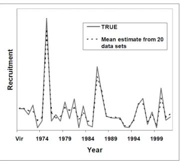
Likewise, the true annual recruitment strongly resembles the mean estimated from the twenty bootstrapped datasets. Although, it is evident that the average estimate of recruitment slightly undershoots the true range of variability, as expected for a model with imperfect data (Figure 2).

(27)

Figure 2. The true recruitment and the average estimated recruitment from 20 bootstrapped data-sets.

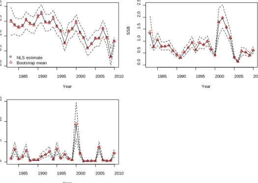
Finally, the parametric estimate of variance in spawning-stock biomass was esti-mated from the inverse Hessian within ADMB and compared to the variability among the fits to the 20 bootstrapped dataset. The results were quite similar, suggest-ing that SS properly characterized the variability in the simulated data (Figure 3).

Figure 3. The parametric estimate of variance in SSB estimated from ADMB’s inverse Hessian is nearly identical with the variability among the fits to the 20 datasets.

Tests Conducted By Others

Numerous tests have been conducted using this model. Those published in peer re-viewed literature include Yin and Sampson (2004), which reached the conclusion that “For all the output variables examined the estimates appeared to be median-unbiased”,wq and Schirripa et al. (2009) which focused on incorporating climate data,

(28)

but provided an additional check of the ability of the model to estimate parameters using simulated data.

Various ongoing research projects have determined that SS is generally capable of estimating parameters used to simulate data. These include the work of Maunder et al. (2009) and separate projects being conducted by Ian Taylor, Tommy Garrison, and Chantel Wetzel, all associated with the University of Washington.

2.3.2 Summary of WKADSAM discussion

Rick Methot presented the Stock-Synthesis (SS) stock assessment method. The key discussion points raised following the presentation were:

• In the first simple example, it was clarified that landings and discards were combined for the simple model.

• In the process example, there were large differences in the size of age 4’s kept in the catch vs. discarded. It was mentioned that there was size-based age sampling.

• With time-varying growth, if fish are greater than Linf (when in changes)

then the fish are modelled to not grow any further.

• In the Grouper example, it was questioned if the switch from female to male was density-dependent? The response was no, but they are close to doing this.

• Propagation of uncertainty. SS includes uncertainty in forecasted quanti-ties.

• Clarified that F is for total catch, and in the model the catch is decomposed into retained and discarded, and the retained model catch is fitted to ob-served catch.

• Morphs and sub-morphs. Morphs are a group of fish with different bio-logical characteristic. Sub-morphs are nested within morphs.

• The index error must be supplied to SS, but there is an option to estimate extra variance for indices.

• A difficult issue is: how do you know when to stop modelling the proc-esses that generate the data? R. Method responded that he would like to see assessments evolve so that the data decides model structure. Also, models need to become more spatially explicit.

• There was discussion on how easy SS could be implemented in the ICES context. The model is very flexible, but there is a penalty attached to this. Some ICES stock assessment scientists only do stock assessment 2 weeks a year, and in this case it is difficult to build and maintain competency with the method. Also, the model flexibility means there are many subjective decisions to make and the assessment can become subjective. R Method suggested that stock assessments should have research models and pro-duction assessment models. The assessment model complexity issue is very real. SS should start off as a research model and not an assessment production model. What we learn about processes from SS is important when understanding other models.

• It was noted that there is a connection between the ‘stiffness’ of models and bias and retrospective problems. However, flexible models can explain residual patterns in different ways. How can we deal with this? R. Method

(29)

agreed. Different communities treat this differently (i.e. assume M, or flat selectivity), and too many fixes may mean the data cannot be fitted.

• Users with agendas can use flexibility to suit their agenda. There is no good answer for this. Also, review panels are also an issue; they change things and sometimes don’t have a good understanding of the changes. • SS is complex, but a particular assessment does not have to be complex.

Many of SS options can be turned off. R. Method agreed, and suggested users take a hierarchical approach, and start simple first.

• SS can do a length-based analysis, but is it better to just code this up your-self. Which is better? Scalability is important. Paring of simple and more detailed models is important.

• There is a danger of over-fitting with a detailed model.

• We have gone to more complex models over the years to better account for uncertainty. But it is difficult to account for uncertainty in more complex models. Should we only build models that we can accurately account for uncertainty for (i.e. using MCMC, etc)? R. Method suggested that this changes over time, and it is a trade-off.

• One desirable feature of simple/stiff models is that you are consistent over time. With flexible models there can be less consistency.

• Can SS be used to explore source of retrospective patterns? R. Method re-plied that the model allows user to cover the sources, and this should be done.

2.4 MULTIFAN-CL

2.4.1 Description

No summary of the model package was provided by the presenter. Rapporteur’s summary of presentation

The presenter started by saying he was giving just a flavour of Multi-fan and what it was designed for and what it can and cannot do. It has been designed for highly mi-gratory species. He will talk about some of the auxiliary software developed for pro-jections and such.

Some of the main challenges are because of large spatial scales, incomplete mixing, and often migratory behaviour. They need to take in to account the effects of spatially explicit fishing in different areas with often different fleet practices that have changed over time. One of the first problems is the lack of catch-at-age data because they are difficult to age. There are strong seasonal patterns, because many of the fish are tropical and only go into far southern and far northern latitudes in specific parts of the year. Catch-reporting by fleet varies, and it could be in weight or length. They have individual weights for some of the higher value fish. Some species have indi-vidual weights for up to 95% of the data. Some fisheries have no data at all. There are no surveys, so tagging data are the main fishery-independent data source. There is high dimensionality in the model because of the diverse data sources.

Multi-fan CL is a combination of two historical approaches, the original Fournier et al MULTIFAN and the Fournier and Archibald approach, which gives MULTIFAN-CL in Fournier et al. 1998. We are still using it 12 years later, and it is the same basic structure.

(30)

The main features include: It uses catch and effort data separately, not cpue. This helps accommodate missing values for when you have one and not the other. It can include temporal CVs for catch/effort data similar to SS. Catch can be in weight or numbers, but not different in same fishery. The catch can be either known exactly or with assigned CVs. Length and/or weight frequency data can be used. Only conven-tional tag data used now, but they are working toward using archival tag data for spatially explicit models.

An example of length frequency data were shown, showing cohorts moving through time. The red lines are different cohort ages.

Tagging data were shown for skipjack tuna. The tagging data are used to help esti-mate both movement and exploitation rate, but not used for growth.

One thing he missed is that it is an age structured model, but uses lengths to estimate those ages. The population dynamics include multi-region and many different time-steps. Seasonal and age-dependent movement is possible but not currently used. One thing to explore is whether movement is time-invariant. What we find is that tropical tunas have different movements because of events like El Niño. One thing they are considering doing is adding covariates for time-dependent movement. Growth is an example of using different time-steps. They also take advantage of the ability to use different growth because of age, such as using LVB for older and Schnute-Richards for early ages. Non-equilibrium initial conditions are possible by estimating an ex-ploitation parameter prior to catch data. A B-H spawner-recruitment curve or inde-pendent recruitment could be used. An environmental recruitment index could be used.

An example of spatial structure was shown where maps showed structure of bigeye tuna, which is divided into six regions. The upper right quadrant showed regional movement patterns. Our plotting function gives different thicknesses, but they do not mean anything here because all movement parameters are the same at age in this model. The estimates of movement are one of the more interesting parts of the as-sessment because of the political implications. The figure in the bottom right quad-rant showed estimates of total biomass over time by region. This can help look at ideas like range contraction. It is easier to estimate movement w/ tagging data, but northern areas can be estimated for movement because they disappear in some sea-sons. The question was asked whether the movement rates were the same for all ages. In this assessment they do not vary by age-classes but they could. The question was asked how the model knows the fish are not there if there is not any fishing. The pre-senter said there is some fishing all year. They could be constant and age-dependent and maybe changed in the future. In MF there are two ways that a fish could be in another region, move there or recruit there. This is confounded in the model because the process could happen either way, so the model does not know this. There are some interesting things that could be done like examining localized spawner-recruit events. We know that tropical tunas spawn continuously given that conditions are favourable. The pie-charts on the figure on the left present catch by gear type. Some fisheries fish when they are 12 inches, intermediate, or large.

The presenter discussed some biological processes. There is some different variation in age-at length in the early years where it departs from LVB. They model natural mortality as a U-shaped distribution quarterly. The large amount of tagging data allows quite consistent estimates of M at age. The estimates range from 0.8 to 0.2 at age 10 and back to 0.6 at age 15.