Bayesian Optimization with Parallel Function Evaluations and Multiple Information Sources: Methodology with Applications in Biochemistry, Aerospace Engineering, and Machine Learning

(1)

BAYESIAN OPTIMIZATION WITH PARALLEL

FUNCTION EVALUATIONS AND MULTIPLE

INFORMATION SOURCES: METHODOLOGY WITH

APPLICATIONS IN BIOCHEMISTRY, AEROSPACE

ENGINEERING, AND MACHINE LEARNING

A Dissertation

Presented to the Faculty of the Graduate School of Cornell University

in Partial Fulfillment of the Requirements for the Degree of Doctor of Philosophy

by Jialei Wang January 2017

(2)

c

(3)

BAYESIAN OPTIMIZATION WITH PARALLEL FUNCTION EVALUATIONS AND MULTIPLE INFORMATION SOURCES: METHODOLOGY WITH APPLICATIONS IN BIOCHEMISTRY, AEROSPACE ENGINEERING, AND

MACHINE LEARNING Jialei Wang, Ph.D. Cornell University 2017

Bayesian optimization, a framework for global optimization of expensive-to-evaluate functions, has recently gained popularity in machine learning and global optimization because it can find good feasible points with few function evalua-tions. In this dissertation, we present novel Bayesian optimization algorithms for problems with parallel function evaluations and multiple information sources, for use in machine learning, biochemistry, and aerospace engineering applications.

First, we present a novel algorithm that extends expected improvement, a widely-used Bayesian optimization algorithm that evaluates one point at a time, to settings with parallel function evaluations. This algorithm is based on a new eﬃcient solution method for finding the Bayes-optimal set of points to evaluate next in the context of parallel Bayesian optimization. The author implemented this algorithm in an open source software package co-developed with engineers at Yelp, which was used by Yelp and Netflix for automatic tuning of hyperparame-ters in machine learning algorithms, and for choosing paramehyperparame-ters in online content delivery systems based on evaluations in A/B tests on live traﬃc.

Second, we present a novel parallel Bayesian optimization algorithm with a worst-case approximation guarantee applied to peptide optimization in biochem-istry, where we face a large collection of peptides with unknown fitness prior to

(4)

experimentation, and our goal is to identify peptides with a high score using a small number of experiments. High scoring peptides can be used for biolabel-ing, targeted drug delivery, and self-assembly of metamaterials. This problem has two novelties: first, unlike traditional Bayesian optimization, where the objective function has a continuous domain and real-valued output well-modeled by a Gaus-sian Process, this problem has a discrete domain, and involves binary output not well-modeled by a Gaussian process; second, it uses hundreds of parallel function evaluations, which is a level of parallelism too large to be approached with other previously-proposed parallel Bayesian optimization methods.

Third, we present a novel Bayesian optimization algorithm for problems in which there are multiple methods or “information sources” for evaluating the ob-jective function, each with its own bias, noise and cost of evaluation. For example, in aerospace engineering, to evaluate an aircraft wing design, diﬀerent computa-tional models may simulate performance. Our algorithm explores the correlation and model discrepancy of each information source, and optimally chooses the in-formation source to evaluate next and the point at which to evaluate it. We describe how this algorithm can be used in general multi-information source opti-mization problems, and also how a related algorithm can be used in “warm start” problems, where we have results from previous optimizations of closely related ob-jective functions, and we wish to leverage these results to more quickly optimize a new objective function.

(5)

BIOGRAPHICAL SKETCH

Jialei Wang was born and raised in Qidong, in JiangSu Province, China, a small but beautiful city by the East China Sea and the Yangtze River. Before he went to college, he spent most of his time in his hometown. After graduating from the high school, he wanted to start a new venture away from the place that he was too familiar with, and in 2007, he went to Nanyang Technological University in Singapore to study Physics. He then transferred to the University of Illinois at Urbana-Champaign, from which he received a B.Sc. in Physics with the highest honors in 2011. In the same year, he joined the Ph.D. program in Applied Physics at Cornell University. In the summer of 2012, he began to work with Professor Peter I. Frazier from the department of Operations Research, and later on, he realized that Operations Research was the right field for him. Professor Peter I. Frazier also became his adviser, and supervised the work in this dissertation.

(6)

To my wife, Ziqi.

It is your constant love and support, that made this work possible.

(7)

ACKNOWLEDGEMENTS

I am grateful to many people for their help in completing my Ph.D.

First and foremost, I would like to thank my adviser, Professor Peter I. Frazier, for constantly helping me to grow both as a researcher and a person. His ability to apply Operations Research to problems from very different fields and collaborate with people from very different background amazes me and sets a great example for me, that continues to encourage me to apply Operations Research to a broader area of problems going forward. His untiring availability for guiding my research and offering advice in cracking problems along the road, made it possible for com-pleting this dissertation work. I also thank Peter, for his generosity in funding my entire Ph.D. research, including attending research conferences, and providing computational resources for conducting numerical experiments.

I am also grateful to my family. I would like to thank my wife, Ziqi, for her constantly caring and support. Failures and stress frequently occur in the journey of doing research, and while I was being upset, it was always Ziqi’s encouragement that brought me back on track, and motivated me until I saw the dawn of success. I also thank my parents, for raising me with great care, oﬀering me the best education opportunities, and setting me a great example through the way they live their lives.

Finally, I would like to thank everyone at Cornell, in particular within my department of Operations Research & Information Engineering, for the marvelous atmosphere of kindness and intelligence they have created. I am grateful to my minor advisers, Professor Thorsten Joachims and Professor Paulette Clancy, for their valuable inputs to this dissertation work. I would also like to thank my research collaborators, for their hard working and great teamwork on the challenges we have taken on.

(8)

LIST OF TABLES

(11)

LIST OF FIGURES

1.1 Illustration of Gaussian process regression with noise-free evalua-tions. The circles show previously evaluated points, (x(i)_{, f}₍_x(i)_)). The solid line shows the posterior mean,µ(n)(x) as a function of x, which is an estimate f(x), and the dashed lines show a Bayesian credible interval for each f(x), calculated as µ(n)₍_x₎±₁_.₉₆_σ(n)₍_x_). Although this example shows f taking a scalar input, Gaussian process regression can be used for functions with vector inputs. . . 8 1.2 Upper panel shows the posterior distribution in a problem with no

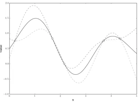
noise and a one-dimensional input space, where the circles are pre-viously sampled points, the solid line is the posterior meanµ(n)₍_x_), and the dashed lines are at µ(n)₍_x₎±₂_σ(n)₍_x_{). Lower panel shows} the probability of improvement PI(x) computed from this poste-rior distribution. Three diﬀerent ϵ values were used in computing probability of improvement to show the eﬀect ofϵin controlling the exploration v.s. exploitation behavior. . . 11 1.3 Upper panel shows the posterior distribution in a problem with no

noise and a one-dimensional input space, where the circles are pre-viously measured points, the solid line is the posterior meanµ(n)(x), and the dashed lines are at µ(n)₍_x₎_±₂_σ(n)₍_x_{). Lower panel shows} the expected improvementEI(x) computed from this posterior dis-tribution. An “x” is marked at the point with the largest expected improvement, which is where we would evaluate next. . . 13 1.4 Upper panel shows the posterior distribution in a problem with

independent normal homoscedastic noise and a one-dimensional in-put space, where the circles are previously measured points, the solid line is the posterior mean µ(n)₍_x_{), and the dashed lines are} at µ(n)(x)±2σ(n)(x). Lower panel shows the natural logarithm of the knowledge gradient factor KG(x) computed from this posterior distribution, where An = An+1 are the discrete grid of 500 points in the range [0,5]. An “x” is marked at the point with the largest KG factor, which is where the KG algorithm would evaluate next. 16 2.1 Expected solution value,f_n∗, vs. iterationn, in the outer

optimiza-tion problem, under MOE-qEI and CL-mix, for three diﬀerent levels of parallelism: q = 2, 4, and 8 threads. We are minimizing, and so smaller function values are better. MOE-qEI converges faster with better solution quality than the heuristic method CL-mix. . . 45 2.2 Expected solution value, f_n∗ vs. iteration n, in the outer

optimiza-tion problem, underEGOand MOE-qEI with diﬀerent levels of par-allelism q. MOE-qEI obtains a substantial speedup over EGO by evaluating in parallel, and the speedup is almost linear in q. . . 46

(12)

2.3 Expected solution quality vs. number of steps in the inner op-timization problem under MOE-qEI and Benchmark 1 (L-BFGS together with the closed form formula for q-EI from [10]). MOE-qEI’s stochastic gradient ascent algorithm converges in fewer steps than L-BFGS in Benchmark 1, and each step is faster. . . 47 2.4 Expected solution quality after 100 steps in the inner

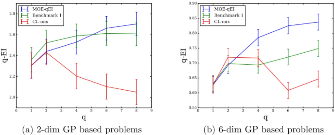
optimiza-tion problem vs. level of parallelism q, under random test prob-lems drawn from a Gaussian process prior in 2 and 6 dimensions. We compare MOE-qEI, Benchmark 1 (L-BFGS together with the closed form formula for q-EI from [10]), and CL-mix. Asq and the dimension increase, MOE-qEI finds higher quality solutions. . . 48 2.5 Average time to compute ∇q-EI with high precision v.s. q,

com-paring the gradient-based estimator from MOE-qEI using a large number of samples (107_{) with the closed-form formula from [61].} The stochastic gradient estimator in MOE-qEI scales better in q

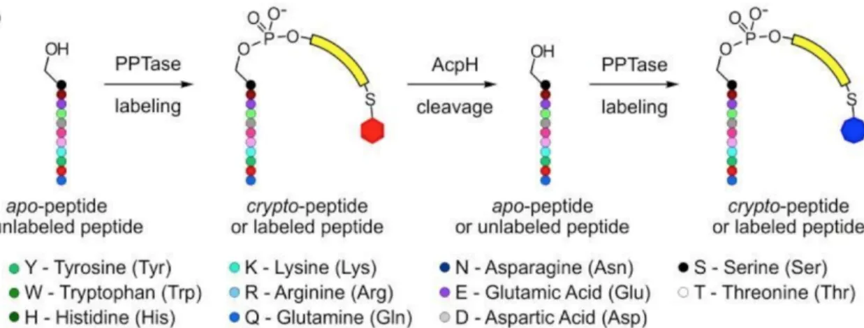
and is faster when q≥4 . . . 51 3.1 Illustration of the reversible labeling process: PPTase modifies the

peptide at a specific Serine residue by addition of a fluorescent molecule, i.e., the labeling process; then AcpH removes this modi-fication, i.e., the unlabeling process. The process can be repeated for many times. . . 54 3.2 ROC curve using leave-one-out cross validation: the left panel is

for classification of sfp activity, the middle panel is for classification of AcpS activity, and the right panel is for classification of AcpH activity. . . 71 3.3 Probability of finding at least one hit from the peptide set

rec-ommended by the three methods: POOL, mutation, and “predict-then-optimize”. The left panel shows the quality of sfp orthogonal peptides, and the right panel shows the quality of AcpS orthogonal peptides. . . 74 3.4 2-dimensional space representation of the peptides recommended

by the three methods and the training dataset, where the “hits” in the training data are marked as red. The left panel shows sfp orthogonal peptides, and the right panel shows AcpS orthogonal peptides. . . 74 3.5 Histogram of hits found in real practice: the left panel shows the

histogram of Sfp-type orthogonal substrates; the right panel shows the histogram of AcpS-type orthogonal substrates. . . 75 4.1 (t) The Rosenbrock benchmark with the parameter setting of [54]:

misoKG oﬀers an excellent gain-to-cost ratio and outperforms its competitors substantially. (b) The Rosenbrock benchmark with the alternative setup. . . 95

(13)

4.2 The performance on the image classification benchmark with sig-nificant model discrepancy. (t) The first 50 steps of each algo-rithm: misoKG and MTBO+ perform better than misoEI. (b) The first 150 steps of misoKG and MTBO+. While the initial perfor-mance of misoKG and MTBO+is comparable,misoKG achieves better testscores after about 80 steps and converges to the global optimum. 98 4.3 The performance on the assemble-to-order benchmark with

signif-icant model discrepancy. misoKG has the best gain per cost ratio among the algorithms. . . 100 4.4 (ul) The basic Rosenbrock function RB1. (ur) The Rosenbrock

function RB2 with an additive sine. (bl) The shifted Rosenbrock functionRB3. (br) The Rosenbrock functionRB4 with an additive sine and a bias depending on x1. . . 103 4.5 (l) ATO 1 (r) ATO 2: All algorithms have the same initial data for

the current problem. wsKG has also access to samples of two runs on related instances, but its hyper-parameters are not optimized for the current instance. . . 104 4.6 (l) ATO 3 (r) ATO 4: wsKG has received the samples of two runs on

(14)

CHAPTER 1 INTRODUCTION

This thesis considers derivative-free global optimization of expensive functions, in which (1) our objective function is time-consuming to evaluate, limiting the num-ber of function evaluations we can perform; (2) evaluating the objective function provides only the value of the objective, and not the gradient or Hessian; (3) we seek a global, rather than a local, optimum. Such problems typically arise when the objective function is evaluated by running a complex computer code (see, e.g., [76]), but also arises when the objective function can only be evaluated by performing a laboratory experiment, or building a prototype system to be evaluated in the real world.

Bayesian optimization (BO) methods constitute one class of methods attempt-ing to solve such problems, where they use machine learnattempt-ing to build a predictive model for the unknown objective function, and then use decision theory to suggest which point(s) in the function’s domain would be the most valuable to evaluate next. Bayesian optimization was pioneered by [53], with early work through the 1970s and 1980s being pursued in [65] and [63]. Development in the 1990s was marked by the popularization of Bayesian optimization by Jones, Schonlau, and Welch, who, building on previous work by Mockus, introduced the Eﬃcient Global Optimization (EGO) method [42]. This method became very popular and well-known in engineering, where it has been adopted for design applications involving time-consuming computer experiments. In the 2000s, development of Bayesian optimization continued in statistics and engineering, and the 2010s have seen ad-ditional development from the machine learning community, where Bayesian opti-mization is used for tuning hyperparameters of computationally expensive machine

(15)

learning models [86]. Other introductions to Bayesian optimization may be found in the tutorial article [8] and textbooks [18, 77], and an overview of the history of the field may be found in [78].

In this chapter, we first collect a few problems arising from engineering and machine learning that are suitable for Bayesian optimization in Section 1.1. We then present the precise problem formulation considered by Bayesian optimization in Section 1.2, and discuss the predictive technique used by Bayesian optimization, called Gaussian Process (GP) regression, in Section 1.2.1, and the methods of suggesting the point(s) to evaluate next in Section 1.2.2. In Section 1.3, we discuss potential usage of Bayesian optimization to the problems in cheminformatics, and additional work need to be done. Finally, we provide an overview for the rest of the thesis in Section 1.4.

1.1

Examples of Bayesian Optimization Problems

Bayesian optimization problems are incredibly common in application. We collect a few examples, arising from engineering and machine learning. Some of these examples will be considered more fully later, and others are included to underscore the broad scope encompassed by the class of Bayesian optimization problems.

• Nano-materials design: We would like to choose design variables to some nano-materials fabrication process to maximize some measure of the per-formance of the design. For example, in the fabrication of nanocrystalline silicon for high-performance / low-power transistor circuit technology, the design variables could be the choice of flow rate, pressure, temperature, ra-diofrequency power, etc., and the performance measure would be the mobility

(16)

of the charge carrier in the transistor channel. Evaluating a design requires making the material and testing it, which takes time, material cost, and manpower. See [45].

• Oil exploration: We would like to discover the best place at which to drill a commercial oil well by drilling a sequence of exploratory test wells. We would like to find a good location with as few exploratory as possible in the discovery process. See [1].

• Drug discovery: We would like to search among chemically similar deriva-tives of a molecule to find the one that best treats a given disease. The number of these molecules is often too large to test all of them in experi-ments, therefore, we test the molecules adaptively, and at each point in time, we decide which molecule to test, and then collect information about its eﬀectiveness. See [66].

• Peptide optimization: We would like to iteratively discover and refine functional peptides with a desired physical / biochemical property, which would support innovations in medicine, biochemistry, and materials science. Few peptides may have the desired property, making the search diﬃcult, because the size of the peptide library to be searched grows exponentially with the maximum peptide length considered. See [24].

• Tuning hyperparameters of machine learning model: For some ma-chine learning algorithms, e.g., deep neural networks, using high-quality hy-perparameters instead of low-quality ones is the diﬀerence between state-of-the-art predictive performance and being essentially useless. Typical ap-proaches to tuning hyperparameters include hand tuning, by experts and brute-force search. However, as the number of parameters grow, these ap-proaches quickly become infeasible. To overcome this challenge, Bayesian

(17)

optimization methods can be used to automate hyperparameter tuning. See [86].

1.2

The Bayesian Optimization Approach

Bayesian optimization considers optimizing a nonlinear functionf(x) over a com-pact setA⊂Rd, formulated concisely as follows:

max

x∈A⊂Rdf(x). (1.1)

In many realistic problems of this kind, we do not know a specific analytic form for the objective function, and can only hope to obtain an estimate of the objective function through simulations or conducting laboratory experiments. Derivative in-formation about the objective functions is not available either. Moreover, sampling fromf(x) is usually an expensive process, for example, conducting an experiment on a new drug design takes days for synthesizing and testing the molecule, com-puting performance metric of a complex machine learning model corresponding to one hyperparameter setting requires hours of computing time, etc. We also assume the problem is non-convex.

Bayesian optimization is particularly suitable for these problems, when the ob-jective function does not have an explicit analytic form, derivative information is not available, and function evaluation is costly. The merit of the Bayesian opti-mization approach stems from two aspects: first, Bayesian optiopti-mization can incor-porate domain expertise about the problem in the form of a Bayesian prior belief; second, the decision-theoretic approach to sampling ensures that each sample is chosen to improve our solution to the optimization problem as much as possible, reducing the number of function evaluations required to find the optimum. We

(18)

will revisit both aspects in Section 1.2.1 and Section 1.2.2.

1.2.1

The Predictive Model: Gaussian Process Regression

Since the objective function is assumed unknown, in Bayesian optimization, we first build a predictive model on the objective function using Bayesian statistics. The name Bayesian comes from the famous “Bayes’ theorem”, which states that the posterior distribution of a random quantity θ given observational data D, is proportional to the likelihood of D given θ multiplied by the prior distribution of

θ:

P(θ | D)∝P(D |θ)P(θ). (1.2) Bayesian models have a few properties that make them well-suited for Bayesian optimization. First, Bayesian models provide a probability distribution over the quantity being predicted, called theposterior, and not just a point estimator. Hav-ing a probability distribution is crucial in Bayesian optimization, as will become clear in Section 1.2.2. Second, Bayesian models make inference about the model parameters based on information obtained from both the observational data and the prespecified prior distribution. Thus one can oﬀer more information than the data itself to the model, by encoding prior knowledge about the model parameters in the prior distribution. Since Bayesian optimization problems typically begin with a small dataset due to the expense of doing function evaluations, Bayesian models’ ability to pool additional information from domain experts helps allevi-ate the “cold start” issue at the beginning of the optimization routine. While optimization methods without Bayesian models may leverage the domain experts’ knowledge by choosing a “good” starting point, it is diﬃcult to more fully encode domain expertise into these methods. In addition, when new observations become

(19)

available, the previous posterior distribution can be used as a prior, and inference logically follow from Bayes’ theorem, allowing convenient updates to Bayesian models, without needing to fully re-train the model on all previous data.

Among the wide variety of Bayesian statistical methods, Gaussian Process (GP) regression is a popular choice in Bayesian optimization. A Gaussian Process is a probability distribution over functions. Under the Gaussian Process, the marginal probability distribution of the value of the function at any single point is a normal distribution. The joint distribution of the values of the function at any collection of points is a multivariate normal distribution.

In Gaussian process regression, we use a Gaussian Process as our prior proba-bility distribution over the unknown objective function. We first place a Gaussian Process prior over the unknown objective functionf, and when data become avail-able, we use Bayes’ theorem to update the posterior, following (1.2), with θ=f.

The detailed specification of the prior, and the updating scheme, is as follows: a Gaussian Process is completely specified by its mean function, µ(x) : A 7→ R, and covariance function,k(x,x′) :A×A7→R. When we place a Gaussian Process prior over the functionf, we write it as

f ∼ GP(µ, k). (1.3)

For a collection of pointsX = (x1, . . . ,xq), the prior of f evaluated at each of the points in X is a multivariate Gaussian distribution

f(X)∼ N (µ(0),Σ(0)), (1.4) where µ(0)_i = µ(xi), and Σ

(0)

ij = k(xi,xj), i, j ∈ {1, . . . , q}. Therefore, µ(0) is a

(20)

of the notations identify which point in the given point collection, while the su-perscript denotes the number of samples observed for updating the posterior. We use the superscript 0 to denote a prior, because at the moment we do not ob-serve any sample. Suppose we have evaluated the objective function at the points

x(1), . . . ,x(n), with the corresponding values y(1), . . . , y(n), and we use x(1:n) and

y(1:n) to simplify the notations, then we can compute the posterior of f over X

using Bayes’ theorem, written as

f(X)|X,x(1:n), y(1:n)∼ N (µ(n),Σ(n)). (1.5) If the function evaluation is noise-free, meaning y(i) = f(x(i)), i = 1, . . . , n, the formula for µ(n) and Σ(n) is

µ(n) =µ(0)+K(X,x(1:n))K(x(1:n),x(1:n))−1(y(1:n)−µ(1:n)),

Σ(n) =K(X,X)−K(X,x(1:n))K(x(1:n),x(1:n))−1K(x(1:n),X),

(1.6)

where µ(1:n) _{is a} _n_{-dimensional vector with each component} _µ(i) ₌ _µ₍_x(i)₎_{, i} ₌ 1, . . . , n; K(X,x(1:n)) _{is a} _q _×_n _{matrix with} _K(_X_,_x(1:n))

ij = k(xi,x

(j)_{), and} similarly forK(x(1:n)_,_X)_, _K₍_X_,_X_{) and} _K(_x(1:n)_,_x(1:n))_.

When function evaluations are noisy, and we assume additive independent iden-tically distributed Gaussian noise with varianceσ2, then we can writeµ(n)andΣ(n) as

µ(n)=µ(0)+K(X,x(1:n)) [K(x(1:n),x(1:n))+σ2I]−1(y(1:n)−µ(1:n)),

Σ(n) =K(X,X)−K(X,x(1:n)) [K(x(1:n),x(1:n))+σ2I]−1K(x(1:n),X).

(1.7) [74, Sect. 2.2] provides the details of the derivation.

Figure 1.1 shows the output from Gaussian process regression on a one-dimensional function. In the figure, circles show points (x(i), f(x(i))), the solid

(21)

Figure 1.1: Illustration of Gaussian process regression with noise-free evaluations. The circles show previously evaluated points, (x(i)_{, f}₍_x(i)_{)). The solid line shows} the posterior mean, µ(n)(x) as a function of x, which is an estimate f(x), and the dashed lines show a Bayesian credible interval for eachf(x), calculated asµ(n)₍_x₎_± 1.96σ(n)₍_x_{). Although this example shows}_f _{taking a scalar input, Gaussian process} regression can be used for functions with vector inputs.

line shows µ(n)(x) as a function of x, and the dashed lines are positioned at

µ(n)(x)±1.96σ(n)(x), forming a 95% Bayesian credible interval for f(x), i.e., an interval in which f(x) lies with posterior probability 95%. (A credible interval is the Bayesian version of a frequentist confidence interval.) Because observations are noise-free, the posterior meanµ(n)₍_x_{) interpolates the observations} _f₍_x_).

[21] oﬀers a comprehensive review of Gaussian process regression, including the choice of mean function and covariance function, inference with noisy observations, and hyperparameters estimation.

(22)

1.2.2

Choosing Where to Sample: Acquisition Functions

for Bayesian Optimization

The second crucial piece of Bayesian optimization is making good decisions about where to direct future sampling. Bayesian optimization methods address this by using a measure of the value of the information that would be gained by sampling at a point, commonly known as an “acquisition function”. Bayesian optimiza-tion methods then choose the point to sample that maximizes this acquisioptimiza-tion function. A number of diﬀerent acquisition functions have been proposed, and here we describe three in detail;probability of improvement [53], expected improve-ment [42, 64], and theknowledge gradient [19, 79]. A more comprehensive review of these acquisition functions may be found in [8, 21]. Other acquisition functions not discussed here include entropy search [92], and composite measures involving the mean and the standard deviation of the posterior [38].

Acquisition Function: Probability of Improvement

Considering the setting of noise-free function evaluations, the early work of [53] suggested maximizing the probability of improvement over the best sampled value observed so far, written as

PI(x) = P(f(x)≥f_n∗+ϵ), (1.8) where f_n∗ = maxm_≤nf(x(m)), is the best sampled value at nth iteration, and ϵ is a positive constant that controls how much improvement over the current best sampled value is desired. Recall in (1.5) that if we have not observedf(x) yet,f(x) is a random variable that follows a normal distribution with meanµ(n)₍_x_{) =}_µ(n)

1 , and standard deviationσ(n)₍_x_{) =}(_Σ(n)

1,1 )1

2

(23)

n here means the distribution is a posterior after observing n data points. Then we can write (1.8) as PI(x) = Φ ( µ(n)₍_x₎₋_f∗ n−ϵ σ(n)₍_x₎ ) , (1.9)

where Φ(·) is the standard normal cumulative distribution function.

The choice of ϵis left to users, although [53] suggested that in general ϵshould start with a bigger value at the beginning of the sampling procedure, to ensure enough exploration of the function domain, and gradually decrease to zero toward the end of sampling to engage more eﬀort in exploitation. Several works have studied the empirical impact of choices ofϵ [90, 41, 58].

Figure 1.2 shows the behavior of probability of improvement for a problem with a one-dimensional input space, and the eﬀect of varying ϵ. We can see that prob-ability of improvement is largest at locations near the current best sampled value. If we did not introduce ϵ, i.e., we setϵ = 0, the probability of improvement algo-rithm would become identical to pure exploitation, because the point with highest probability of being greater than the current best sampled value would simply be the best previously sampled point, as shown in the figure. To add exploration to the algorithm, we must increase ϵ. When ϵ is large, Figure 1.2 confirms that as we set ϵlarger, the algorithm favors points that have large potential gain over the current best sampled value.

Acquisition Function: Expected Improvement

A more satisfying alternative acquisition function would not only consider the probability of improvement, but also the magnitude of the improvement. [42] proposed such an alternative, called expected improvement. As its name suggests,

(24)

Figure 1.2: Upper panel shows the posterior distribution in a problem with no noise and a one-dimensional input space, where the circles are previously sam-pled points, the solid line is the posterior mean µ(n)₍_x_{), and the dashed lines are} at µ(n)₍_x₎±₂_σ(n)₍_x_{). Lower panel shows the probability of improvement} _PI₍_x₎ computed from this posterior distribution. Three diﬀerent ϵ values were used in computing probability of improvement to show the eﬀect of ϵ in controlling the exploration v.s. exploitation behavior.

the formulation is

EI(x) =En [

(f(x)−f_n∗)+], (1.10) whereEn[·] is the conditional expectation given previousnevaluations. The expec-tation in (1.10) can be written more explicitly, in terms of the normal cumulative distribution function Φ(·), and the normal probability density functionφ(·):

EI(x) = (µ(n)(x)−f_n∗)Φ ( µ(n)(x)−f_n∗ σ(n)₍_x₎ ) +σ(n)(x)φ ( µ(n)(x)−f_n∗ σ(n)₍_x₎ ) . (1.11)

The advantage of this formulation compared with the probability of improve-ment is that, without a user defined controlling variableϵ, the expected

(25)

improve-ment balances trade-oﬀ between exploration and exploitation automatically. In fact, the expected improvement favors points that, on the one hand, have a large predicted value, while on the other hand, have a significant amount of uncertainty to allow room for improvement.

We illustrate this behavior in Figure 1.3, which plots the expected improvement for a problem with a one-dimensional input space. We can see from this plot that the expected improvement is largest at locations where both the posterior mean

µ(n)₍_x_{) is large, and also the posterior standard deviation} _σ(n)₍_x_{) is large. This is} reasonable because those points that are most likely to provide large gains are those points that have a high predicted value, but that also have significant uncertainty. Indeed, at points where we have already observed, and thus have no uncertainty, the expected improvement is 0. This is consistent with the idea that, in a problem without noise, there is no value to repeating an evaluation that has already been performed.

In many applications, e.g., those involving physical experiments or stochastic simulations, measurements are noisy. The formulation (1.10) is not applicable in this case, because (1) f_n∗ is not well-defined under noisy observations, and (2) it does not account for the prediction uncertainty at the current best point. To al-leviate these diﬃculties, alternative formulations of expected improvement were proposed in literature. For example, [39] proposed augmented expected improve-ment, which changed the original formulation of expected improvement to adapt to the noisy setting: (1) it used the Gaussian Process updating equations for noisy measurements, given in (1.7); (2) it defined the current “eﬀective best so-lution” as maxm≤n

(

µ(n)₍_x(m)₎−_c·_σ(n)₍_x(m)₎) _{to replace the original definition of} the current best solution, where c is a constant that can reflect the users’ degree

(26)

Figure 1.3: Upper panel shows the posterior distribution in a problem with no noise and a one-dimensional input space, where the circles are previously measured points, the solid line is the posterior mean µ(n)₍_x_{), and the dashed lines are at}

µ(n)₍_x₎±₂_σ(n)₍_x_{). Lower panel shows the expected improvement}_EI₍_x_{) computed} from this posterior distribution. An “x” is marked at the point with the largest expected improvement, which is where we would evaluate next.

of risk aversion; (3) it discounted the original expected improvement by a factor of (1− √ σ

(σ(n)₍_x₎₎2_+σ2), to account for the diminishing return of additional replicates as the prediction becomes more accurate. In addition to this work, there are other approaches in extending expected improvement to the noisy setting proposed in literature; refer to [40, 68] for detail.

Acquisition Function: Knowledge Gradient

Knowledge gradient [20, 79] fully accounts for the introduction of noise, and makes it possible to search over a class of solutions broader than just those that have been

(27)

previously evaluated when recommending the final solution.

We first introduce a set An, which is the set of points from which we would choose final solution, if we were asked to recommend a final solution at time n, based on x(1:n), y(1:n). For tractability, we suppose An is finite. For example, if A is finite, as it often is in discrete optimization via simulation problems, we could takeAn=A, allowing the whole space of feasible solutions. This choice was considered in [20]. Alternatively, one could take An = x(1:n), stating that one is willing to consider only those points that have been previously evaluated. This choice is consistent with the expected improvement algorithm. Indeed, we will see that when one makes this choice, and measurements are free from noise, then the knowledge gradient algorithm is identical to the expected improvement algorithm. Thus, the knowledge gradient algorithm generalizes the expected improvement algorithm.

If we were to stop sampling at timen, then the expected value of a pointx∈An based on the information available would be En[f(x)] = µ(n)(x). In the special case when evaluations are free from noise, this is equal tof(x), but when there is noise, these two quantities may diﬀer. If we needed to report a final solution, we would then choose the point in An for which this quantity is the largest, i.e., we would choose argmax_x_∈_A_nµ(n)(x). Moreover, the expected value of this solution would be

µ∗_n = max

x∈An

µ(n)(x).

If evaluations are free from noise andAn ={x(1:n)}, thenµ∗n is equal to fn∗, but in general these quantities may diﬀer.

(28)

would report based on this additional information is

µ∗_n+1 = max x∈An+1

µ(n+1)(x),

where as before, An+1 is some finite set of points we would be willing to consider when choosing a final solution. Observe in this expression that µ(n+1)(x) is not necessarily the same asµ(n)(x), even for pointsx∈ {x(1:n)}that we had previously evaluated, but that µ(n+1)₍_x_{) can be computed from the history of observations}

x(1:n+1)_, _y(1:n+1)_.

The improvement in our expected solution value is then the diﬀerence between these two quantities,µ∗_n+1−µ∗_n. This improvement is random at timen, even fixing

x(n+1)_{, through its dependence on} _y(n+1)_{, but we can take its expectation. The} resulting quantity is called the knowledge gradient (KG) factor, and is written,

KGn(x) = En [

µ∗_n+1−µ∗_n|x(n+1) =x]. (1.12)

Calculating this expectation is more involved than calculating the expected improvement, but nevertheless can also be done analytically in terms of the normal pdf and normal cdf. This is described in more detail in [20].

The knowledge gradient algorithm is then the one that chooses the point to sample next that maximizes the KG factor,

argmax

x

KGn(x).

The KG factor for a one-dimensional optimization problem with noise is pic-tured in Figure 1.4. We see a similar trade-oﬀ between exploration and exploita-tion, where the KG factor favors measuring points with a largeµ(n)₍_x_{) and a large}

(29)

Figure 1.4: Upper panel shows the posterior distribution in a problem with inde-pendent normal homoscedastic noise and a one-dimensional input space, where the circles are previously measured points, the solid line is the posterior meanµ(n)₍_x_), and the dashed lines are at µ(n)(x) ±2σ(n)(x). Lower panel shows the natural logarithm of the knowledge gradient factor KG(x) computed from this posterior distribution, where An = An+1 are the discrete grid of 500 points in the range [0,5]. An “x” is marked at the point with the largest KG factor, which is where the KG algorithm would evaluate next.

evaluated, just as with the expected improvement, but because there is noise in our samples, the value at these points is not 0 — indeed, when there is noise, it may be useful to sample repeatedly at a point.

Recall that the KG factor depends on the choice of the sets An and An+1. For noise-free problems, if we set An+1 = {x(1:n+1)} and An = {x(1:n)}, we will see that the KG factor recovers expected improvement. Typically, to achieve a better result, we choose these sets to contain more elements, allowing µ∗_n and µ∗_n+1 to

(30)

range over a larger portion of the space, and allowing the KG factor calculation to more accurately approximate the value that would result if we implemented the best option. However, the trade-oﬀ is that as we increase the size of these sets, computing the KG factor is slower, making implementation of the KG method more computationally intensive.

1.3

Bayesian Optimization for Cheminformatics

Cheminformatics is an interdisciplinary field that combines chemistry, computer science and information science, and has received much attention in the past decade. The primary application of Cheminformatics includes virtual screening of libraries of chemical compounds for identifying functional molecules [49, 80]. For example, pharmaceutical companies use the virtual screening techniques to preselect and narrow down candidate compounds in the process of drug discovery.

Machine learning plays a substantial role in Cheminformatics, and in particu-lar, the researchers can use machine learning prediction of the molecular activities, to eﬃciently guide their experimental evaluation in the search for the functional molecules of interest. In this context, machine learning researchers have compared two approaches: (1) evaluate the molecules with the best predicted performance according to the trained machine learning model (the so-called “pure exploitation” approach); (2) evaluate the molecules having the most potential to improve over the best previously evaluated molecule (the Bayesian optimization approach). Al-though the Bayesian optimization approach has shown its superior performance over the “pure exploitation” approach in a variety of experimental design appli-cations [26, 9, 86], Bayesian optimization has been pursued only in a limited way

(31)

in Cheminformatics [66, 56], the majority of work leveraging machine learning for searching functional molecules has used pure exploitation [2, 81, 6].

To apply Bayesian optimization to a broader range of Cheminformatics appli-cations, we need additional work: first, the Gaussian process regression method we have discussed in Section 1.2.1 assumes the objective function is continuous, while in Cheminformatics applications, the search space is usually discrete. This problem has been addressed by [66], where they proposed a linear additive model to predict the measure of molecular activity. However, the sampling policy in this work is only computationally feasible for a limited number of candidates (typically less than 107_{). Second, the response value is not always a scalar. For instance,} high throughput screening, a popular technique in drug screening, reports whether the candidate molecule is “active hit” or not, which is a binary response. Third, it is incredibly common to examine hundreds to thousands of molecules in paral-lel in Cheminformatics applications. Although there are a few works in Bayesian optimization with applications to other fields [86, 26, 94], and work in active learn-ing [9], that proposed parallel sampllearn-ing strategies, none of the methods handles discrete function domain or binary response. To this end, we propose a novel discrete Bayesian optimization method, which we will discuss in Chapter 3.

1.4

Thesis Organization

This thesis is built upon the author’s previously published works: the review of Bayesian optimization in Section 1.2 can be found in [21]; Chapter 2 is based on [94]; Chapter 3 is based on a working paper by the author, which is being prepared for journal submission at the time of completing this thesis; Chapter 4 is

(32)

based on [69] and [70]. We now give an overview of each chapter as follows:

Chapter 2

Chapter 2 considers parallel Bayesian optimization, and proposes an eﬃcient method based on stochastic approximation for implementing a conceptual Bayesian optimization algorithm proposed by [26]. To accomplish this, Chapter 2 uses in-finitesimal perturbation analysis (IPA) to construct a stochastic gradient estimator and shows that this estimator is unbiased. Chapter 2 also shows that the stochas-tic gradient ascent algorithm using the constructed gradient estimator converges to a stationary point of the q-EI surface, and therefore, as the number of multi-ple starts of the gradient ascent algorithm and the number of steps for each start grow large, the one-step Bayes optimal set of points is recovered. Chapter 2 shows in numerical experiments that the method for maximizing the q-EI is faster than methods based on closed-form evaluation using high-dimensional integration, when considering many parallel function evaluations, and is comparable in speed when considering few. Chapter 2 also shows that the resulting one-step Bayes optimal algorithm for parallel global optimization finds high quality solutions with fewer evaluations than a heuristic based on approximately maximizing the q-EI. A high quality open source implementation of this algorithm is available in the open source Metrics Optimization Engine (MOE).

Chapter 3

Chapter 3 consider a discrete Bayesian optimization problem arising in biochem-istry, in which we wish to find a peptide that (1) has a certain expensive-to-ascertain biochemical property (it is a substrate for two protein-modifying

(33)

en-zymes, phosphopantetheinyltransferase and ACP hydrolase); and (2) is as short as possible. Finding such a peptide would allow tracking protein interactions with great ease, and would support a number of innovations in medicine, biochemistry, and materials science. However, such peptides are diﬃcult to find, because the set of peptides is large, only a small fraction have the desired property, and as-certaining whether or not a peptide has the desired property requires performing a time-consuming laboratory experiment. Chapter 3 presents a novel Bayesian optimization method for choosing which peptides to test to find such a peptide as quickly as possible. Chapter 3 proves theoretical bounds on its solution quality, demonstrates in simulation that it outperforms two natural benchmark methods, and then describes how it was used in practice to find a peptide with the desired property that is shorter than the shortest previously known. While the method was developed for this specific application in biochemistry, it can also be used in other discrete Bayesian optimization problems in which we wish to find an exem-plar whose expensive-to-obtain binary label is positive, and for which a secondary easy-to-evaluate cost objective is as small as possible.

Chapter 4

Chapter 4 considers two closely related problems in Bayesian optimization: the first is called multi-information source optimization problem, or MISO, where the goal is to optimize an expensive-to-evaluate black-box function, and in addition to evaluating the objective function directly, there are multiple cheap approximate estimates of the objective that we could use, the so-called “information sources”. This scenario typically arises in engineering sciences. For example, in aerospace en-gineering, when designing an airfoil, there are various computer simulators, based on diﬀerent physical models and with diﬀerent fidelity, to evaluate the

(34)

perfor-mance of a design. The computer simulators in this context, are information sources, where some of them are more computationally expensive and may provide more accurate estimate, while the cheaper information sources may only offer a crude estimate with much less computational cost. The goal is to efficiently utilize the information sources and reduce the overall cost during the optimization task. The second problem is called warm starting Bayesian optimization, which aims to speedup the optimization routine using additional information from previously solved related problems. This scenario typically occurs when one solves a series of optimization problems, where the objective functions are from the same family but with variations. For example, decision making problems that use one optimization model and input data collected over different time periods, are interrelated.

Both problems are similar in that there are multiple “sources” that are closely related to the optimization objective, and are cheaper to query than the original objective. Chapter 4 proposes a novel Bayesian model that specifically analyzes the correlation structure among the “sources”, and then presents a cost-sensitive Knowledge Gradient algorithm that makes optimal decision in choosing both which point to sample and using which “source”.

Chapter 5

Chapter 5 summarizes the contributions of this thesis and describes ongoing work in Bayesian optimization known to this author. In particular, it describes prospec-tive problems in biochemistry and engineering, where the Bayesian optimization techniques developed in this thesis are being used or have potential usage, and new methodological work in parallel Bayesian optimization and multi-information source Bayesian optimization.

(35)

CHAPTER 2

PARALLEL BAYESIAN OPTIMIZATION OF EXPENSIVE FUNCTIONS

2.1

Introduction

The traditional Bayesian optimization procedures, including the methods we have discussed in Chapter 1, are all sequential, which means we iteratively sample one point at a time. In the recent years, with the advance of technology in many ar-eas, parallelization is becoming increasingly popular, and sometimes crucial to the feasibility of a problem. For example, in computational science and engineering, the advent of multi-core computing speeds up the computation in wall clock time, making it essential in time sensitive tasks. In drug discovery, the research lab needs to make a lot of candidate molecules and test individually, which is extremely time consuming; with the introduction of robotics and automation, one can test hun-dreds of candidates at the same time, and speed up the process significantly. Then it is natural to ask how we can parallelize our Bayesian optimization procedures. This chapter proposes a novel parallel Bayesian optimization method, which is a generalization of expected improvement to its parallel setting.

The expected improvement algorithm, known asEGO[42], chooses each point at which to evaluate the expensive objective function in the “outer” expensive global optimization problem, i.e., the problem in (1.1), by solving an “inner” optimization problem: maximize expected improvement. If this is the final point that will be evaluated in the outer optimization problem, and if additional conditions are satisfied (the evaluations are free from noise, and the implementation decision, i.e., the solution that will be implemented in practice after the optimization is

(36)

complete, is restricted to be a previously evaluated point), then the point with largest expected improvement is the Bayes-optimal point to evaluate, in the sense of providing the best possible average-case performance in the outer expensive global optimization problem [21].

The notion of expected improvement was generalized by [26] to the parallel setting, in which the expensive objective can be evaluated at several points simul-taneously. This generalization, called the “multi-points expected improvement” or the q-EI, is consistent with the decision-theoretic derivation of expected improve-ment, and quantifies the expected utility that will result from the evaluation of a

set of points. [26] also provided an analytical formula for the case whenq = 2, or 2-EI.

If the generalized inner optimization problem proposed by [26], which is to find the set of points to evaluate next that jointly maximize the q-EI, could be solved eﬃciently, then this would provide the one-step Bayes-optimal set of points to eval-uate in the outer problem, and would create a one-step Bayes-optimal algorithm for global optimization of expensive functions able to fully utilize parallelism.

This generalized inner optimization problem is challenging, however, because unlike the (scalar) expected improvement used by EGO, which has an easy-to-compute and easy-to-diﬀerentiate expression as shown in (1.11), the q-EI lacks an easy-to-compute expression, and is calculable only through Monte Carlo sim-ulation, dimensional numerical integration, or expressions involving high-dimensional multivariate normal cumulative distribution functions. This signifi-cantly restricts the set of applications in which a naive implementation can solve the inner problem faster than a single evaluation of the outer optimization problem. Stymied by this diﬃculty, [26], as well as the later work in [10], propose heuristic

(37)

methods that are motivated by the one-step optimal algorithm of evaluating the set of points that jointly maximize theq-EI, but that do not actually achieve this gold standard.

Contributions. The main contribution of the research described in this chap-ter is to provide a method that solves the inner optimization problem of maxi-mizing the q-EI eﬃciently, creating a practical and broadly applicable one-step Bayes-optimal algorithm for parallel global optimization of expensive functions. To accomplish this we use infinitesimal perturbation analysis (IPA) (see [33]) to construct a stochastic gradient estimator of the gradient of the q-EI surface, and show that this estimator is unbiased, with a bounded second moment. Our method uses this estimator within a stochastic gradient ascent algorithm, and we show that it converges to a stationary point of theq-EI surface. We use multiple restarts to identify multiple stationary points, and then use ranking and selection to identify the best stationary point found. As the number of restarts and the number of iter-ations of stochastic gradient ascent within each start both grow large, the one-step optimal set of points to evaluate is recovered.

Our method can be implemented in both synchronous environments, in which function evaluations are performed in batches and finish at the same time, and asynchronous ones, in which a function evaluation may finish before others are done.

In addition to our methodological contribution, we have developed a high-quality open source software package, the “Metrics Optimization Engine (MOE)” [12], implementing our method for solving the inner optimization problem, and the resulting algorithm for parallel global optimization of expensive functions. To

(38)

fur-ther enhance computational speed, the implementation takes advantage of parallel computing, and achieves 100X speedup over single-threaded computation when de-ployed on a graphical processing unit (GPU). This software package has been used by Yelp and Netflix to solve global optimization problems arising in their busi-nesses [11, 4]. For the rest of this chapter, we refer to our method as “MOE-qEI” because it is implemented in MOE.

We compare MOE-qEI against several benchmark methods. We show that MOE-qEI provides high-quality solutions to the outer optimization problem more quickly than the heuristic CL-mix policy proposed by [10], which is motivated by the inner optimization problem. We also show that MOE-qEI provides a sub-stantial parallel speedup over the single-threadedEGOalgorithm, which is one-step optimal when parallel resources are unavailable. We also compare our simulation-based method for solving the inner optimization problem against methods simulation-based on exact evaluation of theq-EIfrom [10] and [61] (discussed in more detail below) and show that our simulation-based approach to solving the inner optimization problem provides solutions to both the inner and outer optimization problem that are comparable in quality and speed whenq is small, and superior when qis large.

Related Work. Developed independently and in parallel with this work is [10], which provides a closed-form formula for computing q-EI, and the book chap-ter [61], which provides a closed-form expression for its gradient. Both require multiple calls to high-dimensional multivariate normal cumulative distribution functions (cdfs). These expressions can be used within an existing continuous optimization algorithm to solve the inner optimization problem that we consider.

(39)

expressions when q is even moderately large is slow and numerically challenging. This is because calculating the multivariate normal cdf in moderately large di-mension is itself challenging, with state of the art methods relying on numerical integration or Monte Carlo sampling as described in [23]. Indeed, the method for evaluating the q-EI from [10] requires q2 evaluations of the q−1 dimensional multivariate normal cdf, and the method for evaluating its gradient requiresO(q4) calls to multivariate normal cdfs with dimension ranging from q − 3 to q. In our numerical experiments, we demonstrate that our method for solving the inner optimization problem requires less computation time and parallelizes more easily than do these competing methods, for q >4, and performs comparably when q is smaller. We also demonstrate that MOE-qEI’s improved performance in the inner optimization problem for q > 4 translates to improved performance in the outer optimization problem.

Other related work includes the previously proposed heuristic CL-mix from [10], which does not solve the inner maximization of q-EI, instead using an approxi-mation. While solving the inner maximization of q-EI as we do makes it more expensive to compute the set of points to evaluate next, we show in our numerical experiments that it results in a substantial savings in the number of evaluations required to find a point with a desired quality. When function evaluations are expensive, this results in a substantial reduction in overall time to reach an ap-proximately optimal solution.

In other related work on parallel Bayesian optimization, [22] and [99] proposed a Bayesian optimization algorithm that evaluates pairs of points in parallel, and is one-step Bayes-optimal in the noisy setting under the assumption that one can only observe noisy function values for single points, or noisy function value diﬀerences

(40)

between pairs of points. This algorithm, however, is limited to evaluating pairs of points, and does not extend to a higher level of parallelism.

There are also other non-Bayesian algorithms for derivative-free global opti-mization of expensive functions with parallel function evaluations from [13, 46] and [36]. These are quite diﬀerent in spirit from the algorithm we develop, not being derived from a decision-theoretic foundation.

Outline of this Chapter. With Gaussian Process regression and expected im-provement already been discussed in Chapter 1, we begin in Section 2.2 by defining the q-EI and the one-step optimal algorithm. We construct our stochastic gradi-ent in Section 2.3.2, and combine this estimator together with stochastic gradigradi-ent ascent to define a one-step optimal method for parallel Bayesian global optimiza-tion in Secoptimiza-tion 2.3.3. Then in Secoptimiza-tion 2.4.1 we show that the constructed gradient estimator of the q-EIsurface is unbiased under certain mild regularity conditions. Moreover, in Section 2.4.2 we provide convergence analysis of the stochastic gra-dient ascent algorithm. Finally, in Section 2.5 we present numerical experiments: we compare MOE-qEI against previously proposed heuristics from the literature; we demonstrate that MOE-qEI provides a speedup over single-threaded EGO; we show that MOE-qEI is more eﬃcient than optimizing evaluations of theq-EIusing closed-form formula provided in [10] whenq is large; and we show that MOE-qEI computes the gradient of q-EI faster than evaluating the closed-form expression proposed in [61].

(41)

2.2

Multi-points Expected Improvement (

q-EI

)

In a parallel computing environment, we wish to use the posterior distribution given by (1.5) to choose the set of points to evaluate next. [26] proposed making this choice using a decision-theoretic approach, in which we consider the utility that evaluating a particular candidate set of points would provide, in terms of their ability to reveal points with objective function values better than previously known. We review this decision-theoretic approach here, and then present a new algorithm for implementing this choice in the next section.

Let q be the number of function evaluations that we may perform in parallel, and let X be a candidate set of points that we are considering evaluating next. Let f_n⋆ = maxm_≤nf(x(m)) indicate the value of the best point evaluated, before beginning these qnew function evaluations. The value of the best point evaluated after allqfunction evaluations are complete will be max (f⋆

n,maxi=1,...,qf(xi)). The diﬀerence between these two values (the values of the best point evaluated, before and after theseqnew function evaluations) is called theimprovement, and is equal to (maxi=1,...,qf(xi)−fn⋆)

+

, wherea+_{= max(}_a,_{0) for} _a∈R_.

We then value a joint set of evaluations at these candidate points X as the ex-pected value of this improvement, and we refer to this quantity as themulti-points expected improvement orq-EI from [26]. This multi-points expected improvement can be written as,

q-EI(X) = En [( max i=1,...,qf(xi)−f ⋆ n )+] , (2.1) where En[·] := E [

·|x(1:n)_{, y}(1:n)] _{is the expectation taken with respect to the} pos-terior distribution.

(42)

[26] then proposes that we should choose to next evaluate the set of points that maximizes the multi-points expected improvement,

argmax

X∈Aq

q-EI(X). (2.2)

In the special case q = 1, which occurs when we are operating without paral-lelism, the multi-points expected improvement reduces to the expected improve-ment, as considered by [63] and [42], and can be evaluated in closed-form, in terms of the normal pdf and cdf. The algorithm that chooses the next point to evaluate according to (2.2) is the EGO algorithm of [42].

[26] provided an analytical calculation of EI when q = 2, but in the same paper Ginsbourger commented that the general case of q-EI has complex expres-sions depending on q-dimensional Gaussian cumulative distribution functions, and computation of q-EI when q is large would have to rely on numerical multivariate integral approximation techniques, which is computationally expensive and makes solving (2.2) diﬃcult. [25] writes “directly optimizing theq-EI becomes extremely expensive as q and d (the dimension of inputs) grow”.

2.3

Algorithm

In this section we present a new algorithm for solving the inner optimization prob-lem (2.2) of maximizingq-EI. This algorithm uses a novel estimator of the gradient of theq-EIpresented in Section 2.3.2, used within a multistart stochastic gradient ascent framework as described in Section 2.3.3. We additionally generalize this technique from synchronous to asynchronous parallel optimization is Section 2.3.4. We begin by introducing some additional notation used to describe our algorithm.

(43)

2.3.1

Notation

In this section we reformulate previously defined equations and define additional notation to better support construction of the gradient estimator.

We first write the posterior distribution onf(X) given by (1.5) in an alternative expression

f(X)=d µ(X) +L(X)Z, (2.3) whereL(X) is the lower triangular matrix obtained from the Cholesky decompo-sition of Σ(n) in (1.5),µ(X) is the posterior mean (identical in meaning toµ(n) in (1.5), but rewritten here to emphasize the dependence onX and deemphasize the dependence onn), and Z is a q-dimensional standard normal random vector.

By substituting (2.3) into (2.1), we have

q-EI(X) =E [( max i=1,...,qei[µ(X) +L(X)Z]−f ∗ n )+] , (2.4)

where ei is a unit vector in direction i and the expectation is over Z. To make (2.4) even more compact, define a new vector m(X) and new matrix C(X),

m(X)i =      µ(X)i−fn∗ if i >0 , 0 if i= 0 , C(X)ij =      L(X)ij if i >0 , 0 if i= 0 , (2.5) and (2.4) becomes q-EI(X) =E [ max i=0,...,qei[m(X) +C(X)Z] ] . (2.6)

(44)

2.3.2

Constructing the Gradient Estimator

We now construct our estimator of the gradient∇q-EI(X). Let

h(X,Z) = max

i=0,...,qei[m(X) +C(X)Z]. (2.7) Then

∇q-EI(X) =∇Eh(X,Z). (2.8) If gradient and expectation in (2.8) is interchangeable, the gradient would be

∇q-EI(X) = Eg(X,Z), (2.9) where g(X,Z) =        ∇h(X,Z) if ∇h(X,Z) exists, 0 otherwise. (2.10)

g(X,Z) can be computed using results on diﬀerentiation of the Cholesky de-composition from [83]. We then propose to use g(X,Z) as our estimator of the gradient ∇q-EI, and will discuss interchangeability of gradient and expectation, which implies unbiasedness of our gradient estimator, in Section 2.4.1. As will be discussed in Section 2.4.2, unbiasedness of the gradient estimator is one of the suﬃcient conditions for convergence of the stochastic gradient ascent algorithm proposed in Section 2.3.3.

2.3.3