R E S E A R C H A R T I C L E
Open Access
Application of an efficient Bayesian discretization
method to biomedical data
Jonathan L Lustgarten
1,2†, Shyam Visweswaran
1*†, Vanathi Gopalakrishnan
1and Gregory F Cooper
1Abstract
Background:Several data mining methods require data that are discrete, and other methods often perform better with discrete data. We introduce an efficient Bayesian discretization (EBD) method for optimal discretization of variables that runs efficiently on high-dimensional biomedical datasets. The EBD method consists of two
components, namely, a Bayesian score to evaluate discretizations and a dynamic programming search procedure to efficiently search the space of possible discretizations. We compared the performance of EBD to Fayyad and Irani’s (FI) discretization method, which is commonly used for discretization.
Results:On 24 biomedical datasets obtained from high-throughput transcriptomic and proteomic studies, the classification performances of the C4.5 classifier and the naïve Bayes classifier were statistically significantly better when the predictor variables were discretized using EBD over FI. EBD was statistically significantly more stable to the variability of the datasets than FI. However, EBD was less robust, though not statistically significantly so, than FI and produced slightly more complex discretizations than FI.
Conclusions:On a range of biomedical datasets, a Bayesian discretization method (EBD) yielded better
classification performance and stability but was less robust than the widely used FI discretization method. The EBD discretization method is easy to implement, permits the incorporation of prior knowledge and belief, and is sufficiently fast for application to high-dimensional data.
Background
With the advent of high-throughput techniques, such as DNA microarrays and mass spectrometry, transcrip-tomic and proteomic studies are generating an abun-dance of high-dimensional biomedical data. The analysis of such data presents significant analytical and computa-tional challenges, and increasingly data mining techni-ques are being applied to these data with promising results [1-4]. A typical task in such analysis, for example, entails the learning of a mathematical model from gene expression or protein expression data that predicts well a phenotype, such as disease or health. In data mining, such a task is called classification and the model that is learned is termed a classifier. The variable that is pre-dicted is called the target variable (or simply the target), which in statistical terminology is referred to as the
response or the dependent variable. The features used in the prediction are called the predictor variables (or simply the predictors), which are referred to as the cov-ariates or the independent variables in statistical terminology.
A large number of data mining methods have been developed for classification; several of these methods are unable to use continuous data and require discrete data [1-3]. For example, most rule learning methods that induce sets of IF-THEN rules and several of the popular methods that learn Bayesian networks require data that are discrete. Some methods that accept continuous data, as for example methods that learn classification trees, discretize the data internally during learning. Other methods, such as the naïve Bayes classifier, that accept both continuous and discrete data, may perform better with discrete data [3,4]. A variety of discretization meth-ods have been developed for converting continuous data to discrete data [5-11], and one that is commonly used is Fayyad and Irani’s (FI) discretization method [9]. * Correspondence: [email protected]
†Contributed equally
1Department of Biomedical Informatics and the Intelligent Systems Program, University of Pittsburgh, Suite M-183 Vale, Parkvale Building, 200 Meyran Avenue, Pittsburgh, PA 15260, USA
Full list of author information is available at the end of the article
© 2011 Lustgarten et al; licensee BioMed Central Ltd. This is an Open Access article distributed under the terms of the Creative Commons Attribution License (http://creativecommons.org/licenses/by/2.0), which permits unrestricted use, distribution, and reproduction in any medium, provided the original work is properly cited.
In this paper, we present an efficient Bayesian discreti-zation method and evaluate its performance on several high-dimensional transcriptomic and proteomic datasets, and we compare its performance to that of the FI dis-cretization method. The remainder of this paper is structured as follows. The next section provides some background on discretization and briefly reviews the FI discretization method. The results section describes the efficient Bayesian discretization (EBD) method and gives the results of an evaluation of EBD and FI on biomedi-cal transcriptomic and proteomic datasets. The final sec-tion discusses the results and draws conclusions.
Discretization
Numerical variables may be continuousordiscrete. A continuous variable is one which takes an infinite num-ber of possible values within a range or an interval. A discrete variable is one which takes a countable number of distinct values. A discrete variable may take few values or a large number of values. Discretization is a process that transforms a variable, either discrete or continuous, such that it takes a fewer number of values by creating a set of contiguous intervals (or equivalently a set of cut points) that spans the range of the variable’s values. The set of intervals or the set of cut points produced by a discretization method is called a discretization.
Discretization has several advantages. It broadens the range of classification algorithms that can be applied to datasets since some algorithms cannot handle continu-ous attributes. In addition to being a necessary pre-pro-cessing step for classification methods that require discrete data, discretization has been shown to increase the accuracy of some classifiers, increase the speed of classification methods especially on high-dimensional data, and provide better human interpretability of mod-els such as IF-THEN rule sets [8,10,11]. The impact of discretization on the performance of classifiers is not only due to the conversion of continuous values to dis-crete ones, but also due to filtering of the predictor vari-ables [4]. Varivari-ables that are discretized to a single interval are effectively filtered out and discarded by clas-sification methods since they are not predictive of the target variable. Due to redundancy and noise in the pre-dictor variables in high-dimensional transcriptomic and proteomic data, such filtering of variables has the poten-tial to improve classification performance. Even classifi-cation methods like Support Vector Machines and Random Forests that handle continuous variables directly and are robust to high dimensionality of the data may benefit from discretization [4]. The main dis-advantage of discretization is the loss of information entailed in the process that has the potential to reduce performance of classifiers if the information loss is
relevant for classification. However, this theoretical con-cern may or may not be a practical one, depending on the particular machine-learning situation.
Discretization methods can be classified as unsuper-vised or superunsuper-vised. Unsuperunsuper-vised methods do not use any information about the target variable in the discreti-zation process while supervised methods do. Examples of unsupervised methods include the Equal-Width method, which partitions the range of variable’s values into a user-specified number of intervals and the Equal-Frequency method, which partitions the range of vari-able’s values into a user-specified fraction of instances per interval. Compared to unsupervised methods, super-vised methods tend to be more sophisticated and typi-cally yield classifiers that have superior performance [8,10,11]. Most supervised discretization methods con-sist of a score to measure the goodness of a set of inter-vals (where goodness is a measure of how well the discretized predictor variable predicts the target vari-able), and a search method to locate a good-scoring set of intervals in the space of possible discretizations. The commonly used FI method is an example of a super-vised method.
A second way to categorize discretization methods is as univariate versus multivariate methods. Univariate methods discretize a continuous-valued variable inde-pendently of all other predictor variables in the data, while multivariate methods take into consideration the possible interactions of the variable being discretized with the other predictor variables. Multivariate methods are rarely used in practice since they are computation-ally more expensive than univariate methods and have been developed for specialized applications [12,13]. The FI discretization method is a typical example of a uni-variate method.
We now introduce terminology that will be useful for describing discretization. Let D be a dataset of n instances consisting of the list ((X1,Z1), (X2,Z2), ..., (Xk, Zk), ..., (Xn,Zn)) that is sorted in ascending order ofXk, where Xk is a real value of the predictor variableX and Zkis the associated integer value of the target variable Z. For example, suppose that the predictor variable represents the expression level of a gene that takes real values in the range 0 to 5.0 and the target variable represents the phenotype that takes the values: healthy or diseased (Z = 0 or Z = 1, respectively). Then, an example datasetDis ((1.2, 0), (1.4, 0), (1.6, 0), (3.7, 1), (3.9, 1), (4.1, 1)). Let Sa, b be a list of the first elements ofD, starting at the athpair inDand ending at the bth pair. Thus, for the above example,S4, 6= (3.7, 3.9, 4.1). For brevity, we denote bySthe list S1,n. LetTbbe a set that represents a discretization of S1, b. For the above example ofD, a possible 2-interval discretization isT6= {S1, 3,S4, 6} = {(1.2, 1.4, 1.6), (3.7, 3.9, 4.1)}. Equivalently,
this 2-interval discretization denotes a cut point between 1.6 and 3.7, and typically the mid-point is chosen, which is 2.65 in this example. Thus, all values below 2.65 are considered as a single discrete value and all values equal or greater than 2.65 are considered another discrete value. For brevity, we denote byTa discretizationTnof S.
Fayyad and Irani’s (FI) Discretization Method
Fayyad and Irani’s discretization method is a univariate supervised method that is widely used and has been cited over 2000 times according to Google Scholar1. The FI method consists of i) a score that is the entropy of the target variable induced by the discretization of the predictor variable, and ii) a greedy search method that recursively discretizes each partition at a cutpoint that minimizes the joint entropy of the two resulting subintervals until a stopping criterion based on the minimum description length (MDL) is met.
For a listSa, bderived from a predictor variableXand a target variableZ that takes J values, the entropyEnt (Sa, b) is defined as: Ent(Sa,b) = J j=1 P(Z=zj)log2P(Z=zj)), (1)
where, P(Z=zj) is the proportion of instances inSa, b where the target takes the value zj. The entropy of Z can be interpreted as a measure of its uncertainty or disorder. Let a cutpointCsplit the listSa, binto the lists Sa, cand Sc+ 1, bto create a 2-interval discretization {Sa, c, Sc + 1,b}. The entropy Ent(C; Sa, b) induced byC is given by: Ent(C;Sa,b) = Sa,c Sa,b Ent(Sa,c) + Sc+1,b Sa,b Ent(Sc+1,b), (2) where, |Sa, b| is the number of instances inSa, b, |Sa, c| is the number of instances in Sa, c, and |Sc+ 1,b| is the number of instances inSc + 1,b. The FI method selects the cut pointCfrom all possible cut points that mini-mizes Ent(C; Sa, b) and then recursively selects a cut point in each of the newly created intervals in a similar fashion. As partitioning always decreases the entropy of the resulting discretization, the process of introducing cut points is terminated by a MDL-based stopping cri-terion. Intuitively, minimizing the entropy results in intervals where each interval has a preponderance of one value for the target.
Overall, the FI method is very efficient and runs inO (n log n) time, where n is the number of instances in the dataset. However, since it uses a greedy search method, it does not examine all possible discretizations and hence is not guaranteed to discover the optimal
discretization, that is, the discretization with the mini-mum entropy.
Minimum Optimal Description Length (MODL) Discretization Method
To our knowledge, the closest prior work to the EBD algorithm, which is introduced in this paper, is the MODL algorithm that was developed by Boulle [5]. MODL is a univariate, supervised, discretization algo-rithm. Both MODL and EBD use dynamic programming to search over discretization models that are scored using a Bayesian measure. EBD differs from MODL in two important ways. First, MODL assumes uniform prior probabilities over the discretization, whereas EBD allows an informative specification of both structure and parameter priors, as discussed in the next section. Thus, although EBD can be used with uniform prior probabil-ities as a special case, it is not required to do so. If we have background knowledge or beliefs that may influ-ence the discretization process, EBD provides a way to incorporate them into the discretization process.
Second, the MODL optimal discretization algorithm has a run time that is O(n3), whereas the EBD optimal discretization algorithm has a run time ofO(n2), where nis the number of instances in the dataset. In essence, EBD uses a more efficient form of dynamic program-ming, than does MODL. Their difference in computa-tional time complexity can have significant practical consequences in terms of which datasets are feasible to use. A dataset with, for example, 10,000 instances might be practical to use in performing discretization using EBD, but not using MODL.
While heuristic versions of MODL have been described [5], which give up optimality guarantees in order to improve computational efficiency, and heuristic versions of EBD could be developed that further decrease its time complexity as well, the focus of the current paper is on optimal discretization.
In the next section, we introduce the EBD algorithm and then describe an evaluation of it on a set of bioin-formatics datasets.
Results
An Efficient Bayesian Discretization Method
We now introduce a new supervised univariate discre-tization method called efficient Bayesian discrediscre-tization (EBD). EBD consists of i) a Bayesian score to evaluate discretizations, and ii) a dynamic programming search method to locate the optimal discretization in the space of possible discretizations. The dynamic pro-gramming method examines all possible discretizations and hence is guaranteed to discover the optimal dis-cretization, that is, the discretization with the highest Bayesian score.
Bayesian Score
We first describe a discretization model and define its parameters. As before, letXandZdenote the predictor and target variables, respectively, letDbe a dataset of n instances consisting of the list ((X1,Z1), (X2, Z2), ..., (Xk, Zk), ..., (Xn, Zn)), as described above, and let S denote a list of the first elements ofD. A discretization modelMis defined as:
M≡ {W,T,},
where,Wis the number of intervals in the discretiza-tion, T is a discretization ofS, andΘis defined as fol-lows. For a specified interval i, the distribution of the target variableP(Z |W=i) is modeled as a multinomial distribution with the parameters {θi 1,θi2,...,θij,...,θiJ} wherejindexes the distinct values of Z. Considering all the intervals,Θ= {θij} over 1≤i≤Iand 1≤j≤ JandΘ specifies all the multinomial distributions for all the intervals in M. Given dataD, EBD computes a Bayesian score for all possible discretizations ofSand selects the one with the highest score.
We now derive the Bayesian score used by EBD to evaluate a discretization modelM. The posterior prob-abilityP(M|D) of Mis given by Bayes rule as follows:
P(M|D) = P(M)·P(D|M)
P(D) , (3)
where P(M) is the prior probability of M, P(D|M) is the marginal likelihood of the dataDgivenM, andP(D) is the probability of the data. SinceP(D) is the same for all discretizations, the Bayesian score evaluates only the numerator on the right hand side of Equation 3 as fol-lows:
Score(M) =P(M)·P(D|M). (4) The marginal likelihood P(D | M) in Equation 4 is derived using the following equation:
P(D|M) =
P(D|M,)P(|M)d, (5)
where Θare the parameters of the multinomial dis-tributions as defined above. Equation 5 has a closed-form solution under the following assumptions: (1) the values of the target variable were generated according to i.i.d. sampling fromP(Z |W=i), which is modeled with a multinomial distribution, (2) the distribution P (Z | W = i) is modeled as being independent of the distributionP(Z|W =h) for all values ofi andhsuch that i ≠ h, (3) for all values i, prior belief about the distribution P(Z |W = i) is modeled with a Dirichlet distribution with hyperparametersaij, and (4) there are
no missing data. The closed-form solution to the mar-ginal likelihood is given by the following expression [14,15]: P(D|M) = I i=1 ⎡ ⎣ (αi) (αi+ni) J j=1 (αij+nij) (αij) ⎤ ⎦, (6) whereΓ(·) is the gamma function,niis the number of instances in the intervali, nijis the number of instances in the interval Wi that have target-valuej, aij are the hyperparameters in a Dirichlet distribution which define the prior probability over the θij parameters, and αi=
J
j=1
αij. The hyperparameters can be viewed as prior counts, as for example from a previous (or a hypothetical) dataset of instances in the intervali that belong to the value j. For the experiments described in this paper, we set all the aijto 1, which can be shown to imply that a prioriwe assume all possible distribu-tions ofP(Z|W=i) to be equally likely, for each inter-vali.2If all aij= 1, then allai=J. With these values for the hyperparameters, and using the fact thatΓ(n) = (n -1)!, Equation 6 becomes the following:
P(D|M) = I i=1 (J−1)! (J−1 +ni)! J j=1 nij! (7)
The term P(M) in Equation 4 specifies the prior probability on the number of intervals and the loca-tion of the cut points in the discretizaloca-tion model M; we call these thestructure priors. The structure priors may be chosen to penalize complex discretization models with many intervals to prevent overfitting. In addition to the structure priors, the marginal likeli-hood P(D | M) includes a specification of the prior probabilities on the multinomial distribution of the target variable in each interval; we call these the para-meter priors. In Equation 6, the alphas specify the parameter priors.
The prior probabilityP(M) is modeled as follows. Let Xk denote a real value of the predictor variable, as described above, and Zkdenote the associated integer value of the target variable. Let Prior(k) be the prior probability of there being at least one cut point between XkandXk + 1. In the Methods section, we describe the use of a Poisson distribution with meanlto implement Prior(k), where l is a structure prior parameter. Con-sider the prior probability for an interval ithat repre-sents the sequence Sai,bi in a discretization modelM. In general, we assume that the prior probability for intervali is independent of the prior probabilities for the other
intervals inM. The prior probability for intervaliin terms of thePriorfunction is defined as follows:
Prior(bi) ⎛ ⎝bi−1 k=ai (1−Prior(k)) ⎞ ⎠. (8)
Expression 8 gives the prior probability that no cut points are present between any consecutive pairs of values of X in the sequence Sai,bi and at least one cut point is present between the values Xbi and Xbi+1. Using the above notation and assumptions, and substituting Equations 7 and 8 into Equation 4, we obtain the spe-cialized EBD score:
Score(M) = I i=1 ⎡ ⎣Prior(bi) ⎛ ⎝bi−1 k=ai (1−Prior(k)) ⎞ ⎠ (J−1)! (J−1 +ni)! J j=1 nij! ⎤ ⎦. (9)
The above score assumes that thenvalues ofX in the dataset Dare all distinct. However, the implementation described below easily relaxes that assumption.
Dynamic Programming Search
The EBD method finds the discretization that maximizes the score given in Equation 9 using dynamic program-ming to search the space of possible discretizations. The pseudocode for the EBD search method is given in Figure 1. It is globally optimal in that it is guaranteed to find the discretization with the highest score. Additional details about the search method used by EBD and its time complexity are provided in the Methods section.
The number of possible discretizations for a predictor variable Xin a dataset withn instances is 2n-1, and this number is typically too large for each discretization to be evaluated in a brute force manner. The EBD method addresses this problem by the use of dynamic program-ming that at every stage uses previously computed opti-mal solutions to subproblems. The use of dynamic programming reduces considerably the number of possi-ble discretizations that have to be evaluated explicitly without sacrificing the ability to identify the optimal discretization.
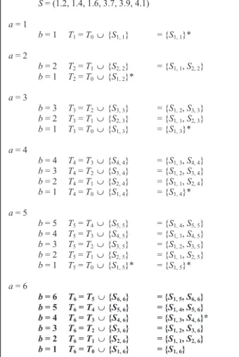
An example of the application of the EBD method on the example datasetD= ((1.2, 0), (1.4, 0), (1.6, 0), (3.7, 1), (3.9, 1), (4.1, 1)) is given in Figure 2. Although there are 25 = 32 possible discretizations for a dataset of six instances, as in this example, EBD explicitly evaluates only 6 of them in determining the highest scoring discretization.
As described in the Methods section, the EBD algo-rithm runs in O(n2) time, where n is the number of instances of a predictorX. Although EBD is slower than FI, it is still feasible to apply EBD to high-dimensional data with a large number of variables.
Evaluation of the Efficient Bayesian Discretization (EBD) Method
We evaluated the EBD method and compared its perfor-mance to the FI method on 24 biomedical datasets (see Table 1) using five measures: accuracy, area under the Receiver Operating Characteristic curve (AUC), robust-ness, stability, and the mean number of intervals per variable (a measure of model complexity). The last three measures evaluate the discretized predictors directly while the first two measures evaluate the performance of classifiers that are learned from the discretized pre-dictors. We performed this comparison using the FI method, because it is so commonly used (1) in practice and (2) as a standard algorithmic benchmark for discre-tization methods.
For computing the evaluation measures we performed 10 × 10 cross-validation (10-fold cross-validation done ten times to generate a total of 100 training and test folds). For a pair of training and test folds, we learned a discretization model for each variable (using either FI or EBD) for the training fold only and applied the intervals from the model to both the training and test folds to gen-erate the discretized variables. For the experiments, we setl, which is user specified parameter introduced in Figure 1 and in Equation 10 (see the Methods section) to be 0.5. The parameterlis the expected number of cut points in the discretization of the variables in the domain. Our previous experience with discretizing some of the datasets used in the experiments with FI indicated that the majority of the variables in these datasets have 1 or 2 intervals (that correspond to 0 or 1 cut points). We chose
lto be 0.5 as the average of 0 and 1 cut points.
We used two classifiers in our experiments, namely, C4.5 and naïve Bayes (NB). C4.5 is a popular tree classi-fier that accepts both continuous and discrete predictors and has the advantage that the classifier can be inter-preted as a set of rules. The NB classifier is simple, effi-cient, robust, and accepts both continuous and discrete predictors. It assumes that the predictors are condition-ally independent of each other given the target value. Given an instance, it applies Bayes theorem to compute the probability distribution over the target values. This classifier is very effective when the independence assumptions hold in the domain; however, even if these assumptions are violated, the classification performance is often excellent, even when compared to more sophis-ticated classifiers [16].
Accuracy is a widely used measure of predictive per-formance (see the Methods section). The mean accura-cies for EBD and FI for C4.5 and NB are given in Table 2. EBD has higher mean accuracy on 17 datasets for each of C4.5 and NB, respectively. FI has higher mean accuracy on 4 datasets and 3 datasets for C4.5 and NB, respectively. EBD and FI have the same mean
accuracy on 4 datasets and 3 datasets for C4.5 and NB, respectively. Overall, EBD shows an increase in accu-racy of 2.02% and 0.76% for C4.5 and NB, respectively. This increased performance is statistically significant at the 5% significance level on the Wilcoxon signed rank test for both C4.5 and NB.
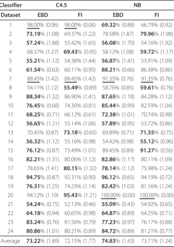
The AUC is a measure of the discriminative perfor-mance of a classifier that accounts for datasets that have a highly skewed distribution over the target variable (see the Methods section). The mean AUCs for EBD and FI for C4.5 and NB are given in Table 3. For C4.5, EBD has higher mean AUC on 17 datasets, FI has higher
Algorithm EBD
Input: Dataset D and parameter Ȝ.
Output: An optimal Bayesian discretization of variable X relative to D.
Definitions of terms:
Let D be a dataset of n instances consisting of the list ((X1, Z1), (X2, Z2), ..., (Xk, Zk), ..., (Xn, Zn)) that is sorted in ascending order of Xk, where Xk is a real value of the predictor variable and Zk is the associated integer value of the target variable.
Let Sa, b be a list of the first elements in D, starting at the ath pair in D and ending at the bth pair. Let Tb be a set that represents a discretization of S1, b.
Let target variable Z have J unique values, and let Zj denote the jth unique value. Let U be a real array of J elements, and let Uj denote its jth element. U will contain the distribution of values of the target variable for some Sa, b.
Let n’ be the number of unique values of predictor variable X, and let Xk denote the kth unique value. Let V be a real array of n’ elements, and let Vy denote its yth element.
For 1 k n’, let Wk = (countk, 1, countk, 2..., countk, J) be an array such that for 1 j J, the term
countk, j is equal to the number of pairs in D in which the first element has value Xk and the second element (i.e., the target value) has value Zj.
Let MarginalLikelihood(U) be the following marginal likelihood function, which follows from Equation 7 when array U is used to derive the ni and nij counts:
1 1 ( 1)! ( ) : ! ( 1 )! J j J j j j J MarginalLikelihood U U J U 1 1)! J 1)! 1)! ((( 11 ! JJ ! J j j J 1 j)! j jjj
Let Prior(k) be the prior function defined in Equation 10 in the text.
Lines of Code: 1. V0 := 1; 2. T0 := {}; 3. for a := 1 to n’ 4. P := Prior(a); 5. Va := 0; 6. U := (0, 0, ..., 0); 7. for b := a downto 1 8. U := U + Wb; /* element-wise addition */ 9. ML := MarginalLikelihood(U); 10. Score_ba := P × ML; 11. if Vb-1 × Score_ba > Va 12. then 13. Ta := Tb-1 {Sb, a}; 14. Va := Vb-1 × Score_ba; 15. P := P × (1 –Prior(b-1)); 16. return Tn’
Figure 1Pseudocode for the efficient Bayesian discretization (EBD) method. The EBD method uses dynamic programming and runs inO (n2) time as indicated by the twoforloops (nis the number of instances in the dataset).
mean AUC on 5 datasets, and both discretization meth-ods have the same mean AUC on 2 datasets. For NB, EBD has higher mean AUC than FI on 16 datasets, lower mean AUC on 6 datasets, and the same mean AUC on two datasets. Overall, EBD shows an improve-ment in AUC of 1.07% and 1.12% for C4.5 and NB, respectively, and both increases in AUC are statistically significant at the 5% level on the Wilcoxon signed rank test.
Robustness is the ratio of the accuracy on the test dataset to that on the training dataset expressed as a percentage (see the Methods section). The mean robust-ness for EBD and FI for C4.5 and NB are given in Table 4. For C4.5, EBD has higher mean robustness on 10 datasets, FI has higher mean robustness on 11 data-sets, and both have equivalent mean robustness on three datasets. For NB, EBD has better performance than FI on 9 datasets, worse performance on 13 data-sets, and similar performance on two datasets. Overall, EBD shows a small decrease in mean robustness of 0.26% and 0.68% for C4.5 and NB, respectively, that are not statistically significant at the 5% level on the Wil-coxon signed rank test.
Stability quantifies how different training datasets affect the variables being selected (see the Methods sec-tion). The mean stabilities for EBD and FI are given in Table 5. Overall, EBD has higher stability than FI, but only at an overall average of 0.02, which nevertheless is statistically significant at the 5% significance level on the Wilcoxon signed rank test.
Input: D = ((1.2, 0), (1.4, 0), (1.6, 0), (3.7, 1), (3.9, 1), (4.1, 1)) S = (1.2, 1.4, 1.6, 3.7, 3.9, 4.1) a = 1 b = 1 T1 = T0 {S1, 1} = {S1, 1}* a = 2 b = 2 T2 = T1 {S2, 2} = {S1, 1, S2, 2} b = 1 T2 = T0 {S1, 2}* a= 3 b = 3 T3 = T2 {S3, 3} = {S1, 2, S3, 3} b = 2 T3 = T1 {S2, 3} = {S1, 1, S2, 3} b = 1 T3 = T0 {S1, 3} = {S1, 3}* a= 4 b = 4 T4 = T3 {S4, 4} = {S1, 3, S4, 4} b = 3 T4 = T2 {S3, 4} = {S1, 2, S3, 4} b = 2 T4 = T1 {S2, 4} = {S1, 1, S2, 4} b = 1 T4 = T0 {S1, 4} = {S1, 4}* a= 5 b = 5 T5 = T4 {S5, 5} = {S1, 4, S5, 5} b = 4 T5 = T3 {S4, 5} = {S1, 3, S4, 5} b = 3 T5 = T2 {S3, 5} = {S1, 2, S3, 5} b = 2 T5 = T1 {S2, 5} = {S1, 1, S2, 5} b = 1 T5 = T0 {S1, 5}* = {S1, 5}* a= 6 b = 6 T6 = T5 {S6, 6} = {S1, 5, S6, 6} b = 5 T6 = T4 {S5, 6} = {S1, 4, S5, 6} b = 4 T6 = T3 {S4, 6} = {S1, 3, S4, 6}* b = 3 T6 = T2 {S3, 6} = {S1, 2, S3, 6} b = 2 T6 = T1 {S2, 6} = {S1, 1, S2, 6} b = 1 T6 = T0 {S1, 6} = {S1, 6} Output: T6 = {S1, 3, S4, 6} = {(1.2, 1.4, 1.6), (3.7, 3.9, 4.1)}
* = discretization with the highest EBD score in iteration a
Figure 2 An example of the application of the efficient Bayesian discretization (EBD) method. This example shows the progression of the EBD method when applying the pseudocode given in Figure 1 to the dataset of six instances that is introduced in the main text. An asterisk denotes the discretization with the highest EBD score in a given iteration, as indexed bya. There are 25 = 32 possible discretizations for a dataset of six instances; for this dataset EBD explicitly evaluates only the 6 discretizations shown in bold font.
Table 1 Description of datasets
Dataset Dataset name Type P/D #t #n #V M 1 Alon et al. T D 2 61 6,584 0.651 2 Armstrong et al. T D 3 72 12,582 0.387 3 Beer et al. T P 2 86 5,372 0.795 4 Bhattacharjee et al. T D 7 203 12,600 0.657 5 Bhattacharjee et al. T P 2 69 5,372 0.746 6 Golub et al. T D 2 72 7,129 0.653 7 Hedenfalk et al. T D 2 36 7,464 0.500 8 Iizuka et al. T P 2 60 7,129 0.661 9 Khan et al. T D 4 83 2,308 0.345 10 Nutt et al. T D 4 50 12,625 0.296 11 Pomeroy et al. T D 5 90 7,129 0.642 12 Pomeroy et al. T P 2 60 7,129 0.645 13 Ramaswamy et al. T D 29 280 16,063 0.100 14 Rosenwald et al. T P 2 240 7,399 0.574 15 Staunton et al. T D 9 60 7,129 0.145 16 Shipp et al. T D 2 77 7,129 0.747 17 Su et al. T D 13 174 12,533 0.150 18 Singh et al. T D 2 102 10,510 0.510 19 Veer et al. T P 2 78 24,481 0.562 20 Welsch et al. T D 2 39 7,039 0.878 21 Yeoh et al. T P 2 249 12,625 0.805 22 Petricoin et al. P D 2 322 11,003 0.784 23 Pusztai et al. P D 3 159 11,170 0.364 24 Ranganathan et al. P D 2 52 36,778 0.556
In the Type column, T denotestranscriptomicand P denotesproteomic. In the
P/D column, P denotesprognosticand D denotesdiagnostic. #t is the number
of values of the target variable and #n is the number of instances in the dataset. #V is the number of predictor variables. M is the proportion of the data that has the majority target value.
Table 6 gives the mean number of intervals obtained by EBD and FI. The first column gives for each dataset the proportion of predictor variables that were discre-tized into a single interval, that is, there were no cut points. Such predictors are considered uninformative and are not used for learning a classifier. The second column gives for each dataset the mean number of intervals among those predictors that were discretized to more than one interval. The third column reports the mean number of intervals over all predictors, including intervals that contain no cut points. Overall, the applica-tion of EBD resulted in more predictors with more than one interval, relative to the application of FI, by an over-all average of 9%. Also, the mean number of intervals per predictor was greater for EBD than for FI, but this difference was not statistically significant at the 5% level on the Wilcoxon signed rank test. This implies that while the average for the EBD complexity is slightly
greater (1.27 versus 1.16 intervals per predictor), overall, EBD and FI are similar in terms of complexity of the discretizations produced.
The results of the statistical comparison of the EBD and FI discretization methods using the Wilcoxon paired samples signed rank test are given in Table 7. As shown in the table, the accuracy and AUC of C4.5 and NB classifiers were statistically significantly better at the 5% level when the predictor variables were discretized using EBD over FI. EBD was statistically significantly more stable to the variability of the datasets than FI. However, EBD was less robust, though not statistically significantly so, than FI and produced slightly more complex discretizations than FI.
Running Times
We conducted the experiments on an AMD X2 4400 + 2.2 GHz personal computer with 2GB of RAM that was running Windows XP. For the 24 datasets included in our study, on average to discretize all the predictor
Table 2 Accuracies for the EBD and FI discretization methods
Classifier C4.5 NB
Dataset EBD (SEM) FI (SEM) EBD (SEM) FI (SEM) 1 100.00% (0.00) 100.00% (0.00) 93.33% (0.93) 93.33% (0.85) 2 86.43% (0.79) 84.62% (0.77) 93.03% (1.06) 92.12% (0.94) 3 78.61% (1.30) 64.23% (1.72) 81.53% (1.11) 81.53% (1.02) 4 88.62% (0.66) 84.38% (0.67) 75.43% (0.83) 72.76% (0.79) 5 59.04% (1.72) 56.33% (1.93) 71.19% (0.92) 69.78% (1.13) 6 96.67% (1.10) 95.67% (0.82) 82.32% (1.17) 80.28% (1.51) 7 94.46% (1.03) 94.46% (1.03) 97.32% (0.84) 97.32% (0.84) 8 60.00% (2.08) 50.00% (2.03) 72.33% (1.42) 70.82% (1.49) 9 83.61% (1.28) 81.29% (0.97) 91.94% (0.91) 93.67% (0.72) 10 68.00% (1.98) 66.54% (1.21) 76.00% (1.65) 71.76% (1.32) 11 77.67% (1.30) 72.44% (0.91) 75.53% (1.33) 73.81% (1.11) 12 55.83% (2.14) 59.58% (2.12) 63.33% (1.81) 61.67% (1.84) 13 58.92% (0.86) 57.14% (0.96) 50.36% (0.84) 49.32% (0.88) 14 58.75% (0.91) 62.33% (1.01) 58.33% (1.04) 57.65% (1.09) 15 54.94% (0.72) 54.20% (0.74) 55.34% (1.70) 53.86% (1.07) 16 72.43% (1.32) 71.25% (1.45) 86.22% (1.41) 85.45% (1.22) 17 70.06% (0.94) 68.96% (1.17) 82.81% (0.79) 81.78% (1.42) 18 81.21% (0.58) 83.78% (0.68) 83.76% (0.91) 89.76% (0.75) 19 74.12% (1.32) 72.22% (1.21) 85.12% (1.09) 84.19% (1.31) 20 59.45% (2.08) 59.45% (2.08) 100.00% (0.00) 100.00% (0.00) 21 62.32% (1.54) 65.24% (1.43) 78.23% (0.59) 76.23% (0.54) 22 73.22% (0.78) 69.78% (1.21) 78.23% (0.77) 77.23% (0.78) 23 73.32% (0.92) 68.49% (0.98) 46.22% (0.98) 48.55% (0.87) 24 76.12% (1.32) 73.04% (1.72) 83.32% (1.65) 80.12% (1.23) Average 73.49% (2.07) 71.48% (2.12) 77.55% (2.65) 76.79% (2.32)
Accuracies for EBD and FI discretization methods are obtained from the application of C4.5 and NB classifiers to the discretized variables. The mean and the standard error of the mean (SEM) for the accuracy for each dataset is obtained by 10 × 10 cross-validation. For each dataset, the higher accuracy is shown in bold font and equal accuracies are underlined.
Table 3 AUCs for the EBD and FI discretization methods
Classifier C4.5 NB
Dataset EBD FI EBD FI 1 98.00% (0.06) 98.00% (0.06) 69.32% (0.88) 66.79% (0.92) 2 73.19% (1.08) 69.37% (1.22) 78.58% (1.87) 79.96% (1.98) 3 57.24% (1.88) 55.42% (1.65) 56.08% (1.70) 54.16% (1.92) 4 68.37% (1.27) 69.43% (0.95) 58.12% (1.08) 59.72% (1.17) 5 55.21% (1.12) 54.38% (1.44) 56.87% (1.41) 53.91% (1.09) 6 61.54% (0.63) 60.11% (0.95) 88.21% (0.66) 86.38% (0.86) 7 88.45% (1.42) 88.45% (1.42) 91.35% (0.76) 91.35% (0.76) 8 54.11% (1.12) 55.49% (0.89) 58.76% (0.85) 59.61% (0.76) 9 88.34% (1.32) 86.90% (1.41) 87.65% (1.18) 84.28% (1.12) 10 76.45% (0.68) 74.30% (0.81) 85.44% (0.99) 82.59% (1.04) 11 68.25% (0.71) 66.12% (0.61) 72.38% (1.01) 70.74% (0.98) 12 56.65% (1.21) 55.14% (1.06) 57.89% (0.95) 53.72% (0.86) 13 70.45% (0.87) 73.18% (0.65) 69.89% (0.71) 71.55% (0.75) 14 56.32% (1.12) 55.16% (0.98) 54.42% (0.98) 55.12% (0.96) 15 76.12% (0.87) 73.49% (1.01) 89.45% (0.89) 91.27% (0.56) 16 82.21% (1.31) 80.06% (1.12) 82.86% (1.17) 80.11% (1.09) 17 78.65% (1.41) 80.15% (1.32) 78.14% (1.12) 75.98% (1.24) 18 94.75% (0.87) 92.31% (0.90) 96.12% (0.65) 94.19% (0.72) 19 76.31% (1.25) 74.23% (1.14) 82.42% (1.03) 81.16% (1.24) 20 94.12% (1.19) 95.43% (1.21) 100.00% (0.00) 100.00% (0.00) 21 54.24% (0.75) 52.13% (0.46) 55.09% (0.43) 54.92% (0.65) 22 64.18% (0.94) 60.65% (0.98) 64.87% (0.89) 64.25% (0.71) 23 83.24% (0.76) 81.56% (0.79) 77.23% (0.97) 76.17% (0.88) 24 80.86% (1.01) 80.21% (0.89) 84.72% (0.89) 81.21% (0.77) Average 73.22% (1.89) 72.15% (1.77) 74.83% (1.43) 73.71% (1.24)
AUCs for EBD and FI discretization methods are obtained from the application of C4.5 and NB classifiers to the discretized variables. The mean and the standard error of the mean (SEM) for the AUC for each dataset is obtained by 10 × 10 cross-validation. For each dataset, the higher AUC is shown in bold font and equal AUCs are underlined.
variables in a dataset, EBD took 20 seconds per training fold while FI took 5 seconds per training fold.
Discussion
We have developed an efficient Bayesian discretization method that uses a Bayesian score to evaluate a discreti-zation and employs dynamic programming to efficiently search and identify the optimal discretization. We evalu-ated the performance of EBD on several measures and compared it to the performance of FI. Table 8 shows the number of wins, draws and losses when comparing EBD to FI on accuracy, AUC, stability and robustness. On both accuracy and AUC, which are measures of dis-crimination performance, EBD demonstrated statistically significant improvement over FI. EBD was more stable than FI, which indicates that EBD is less sensitive to the variability of the training datasets. FI was moderately better in terms of robustness, but not statistically
significantly so. On average, EBD produced slightly more intervals per predictor variable, as well as a greater proportion of predictors that had more than one inter-val. Thus, EBD produced slightly more complex discreti-zations than FI.
A distinctive feature of EBD is that it allows the speci-fication of parameter and structure priors. Although we used non-informative parameter priors in the evaluation reported here, EBD readily supports the use of informa-tive prior probabilities, which enables users to specify background knowledge that can influence how a predic-tor variable is discretized. The alpha parameters in Equation 6 are the parameter priors. Suppose there are two similar biomedical datasets A and B containing the same variables, but different populations of individuals, and we are interested in discretizing the variables. The data in A could provide information for defining the parameter priors in Equation 6 before its application to the data in B. There is a significant amount of flexibility in defining this mapping for using data in a similar (but not identical) biomedical dataset to influence the discre-tization of another dataset. The lambda parameter in
Table 4 Robustness for the EBD and FI discretization methods
Classifier C4.5 NB
Dataset EBD (SEM) FI (SEM) EBD (SEM) FI (SEM) 1 100.00% (0.00) 100.00% (0.00) 94.94% (0.89) 94.94% (0.97) 2 90.64% (0.77) 87.69% (0.86) 94.36% (0.98) 95.17% (1.05) 3 70.78% (2.00) 53.57% (2.10) 82.44% (1.10) 81.69% (1.14) 4 84.18% (0.76) 85.87% (0.77) 90.10% (1.09) 75.91% (1.09) 5 49.83% (2.01) 53.08% (2.18) 69.97% (1.20) 86.88% (1.12) 6 83.58% (1.34) 80.58% (1.42) 97.76% (1.12) 95.89% (0.92) 7 92.50% (1.18) 92.50% (1.18) 96.67% (0.86) 97.27% (0.86) 8 55.50% (2.16) 55.11% (2.06) 70.94% (1.48) 71.67% (1.43) 9 90.61% (0.95) 87.16% (0.99) 98.98% (0.74) 96.08% (0.94) 10 75.10% (1.48) 68.65% (1.39) 74.35% (2.05) 76.93% (1.81) 11 70.36% (0.95) 70.47% (0.93) 78.25% (1.22) 82.52% (1.20) 12 57.82% (2.22) 61.04% (2.21) 63.47% (1.87) 65.94% (1.88) 13 66.12% (0.39) 66.96% (0.37) 64.89% (1.05) 50.83% (1.02) 14 57.47% (0.94) 64.13% (1.06) 67.01% (1.08) 69.18% (1.08) 15 54.94% (0.72) 54.20% (0.74) 54.16% (1.75) 61.60% (1.70) 16 73.17% (1.66) 77.17% (1.79) 92.57% (1.39) 84.11% (1.38) 17 82.71% (1.35) 87.43% (1.21) 88.25% (1.56) 85.49% (1.60) 18 79.38% (0.57) 82.65% (0.57) 88.91% (0.72) 91.81% (0.83) 19 73.00% (1.48) 79.00% (1.30) 85.55% (1.31) 85.89% (1.29) 20 58.75% (2.09) 58.75% (2.08) 100.00% (0.00) 100.00% (0.00) 21 55.18% (1.26) 62.23% (1.13) 77.01% (0.60) 76.10% (0.57) 22 72.53% (0.96) 66.84% (1.03) 90.87% (0.89) 81.15% (0.93) 23 78.16% (1.04) 76.07% (0.99) 77.79% (1.67) 52.49% (1.73) 24 75.00% (1.78) 70.00% (1.75) 80.33% (1.64) 99.86% (1.70) Average 72.55% (2.81) 72.81% (2.76) 81.72% (2.92) 82.40% (2.59)
The mean and the standard error of the mean (SEM) for robustness for each dataset is obtained by 10 × 10 cross-validation. For each dataset, the higher robustness value is shown in bold font and equal robustness values are underlined.
Table 5 Stabilities for the EBD and FI discretization methods Dataset EBD FI 1 0.83 0.80 2 0.84 0.84 3 0.68 0.67 4 0.82 0.84 5 0.54 0.50 6 0.79 0.80 7 0.81 0.79 8 0.58 0.55 9 0.84 0.82 10 0.83 0.81 11 0.80 0.75 12 0.50 0.50 13 0.76 0.78 14 0.53 0.53 15 0.65 0.59 16 0.80 0.79 17 0.81 0.75 18 0.76 0.82 19 0.75 0.69 20 0.88 0.84 21 0.60 0.42 22 0.86 0.85 23 0.89 0.94 24 0.59 0.61 Average 0.74 0.72
The mean stability for each dataset is obtained by 10 × 10 cross-validation. For each dataset, the higher stability value is shown in bold font and equal stability values are underlined.
Table 6 Mean number of intervals per predictor variable for the EBD and FI discretization methods
Mean fraction of predictors with 1 interval Mean # of intervals per predictor with >1 interval Mean # of intervals per predictor
Dataset EBD FI EBD FI EBD FI
1 0.81 0.84 2.02 2.01 1.15 1.16 2 0.47 0.61 2.06 2.04 1.48 1.41 3 0.91 0.96 2.02 2.01 1.05 1.04 4 0.18 0.28 2.20 2.16 1.91 1.84 5 0.97 0.99 2.03 2.04 1.01 1.01 6 0.87 0.89 2.01 2.01 1.13 1.11 7 0.82 0.86 2.02 2.01 1.13 1.14 8 0.97 0.98 2.02 2.02 1.01 1.02 9 0.54 0.76 2.11 2.12 1.42 1.27 10 0.38 0.65 2.06 2.06 1.53 1.37 11 0.51 0.77 2.06 2.10 1.41 1.25 12 0.98 0.99 2.02 2.02 1.01 1.01 13 0.05 0.90 2.57 2.10 2.39 1.11 14 0.98 0.99 2.03 2.02 1.01 1.01 15 0.70 0.98 2.08 2.12 1.20 1.02 16 0.75 0.87 2.01 2.01 1.12 1.13 17 0.76 0.85 2.04 2.04 1.16 1.16 18 0.17 0.78 2.31 2.13 1.99 1.25 19 0.87 0.94 2.05 2.02 1.06 1.06 20 0.81 0.85 2.02 2.10 1.15 1.17 21 0.97 0.99 2.01 2.02 1.01 1.01 22 0.82 0.84 2.14 2.14 1.16 1.18 23 0.93 0.97 2.01 2.02 1.05 1.03 24 0.92 0.95 2.06 2.02 1.04 1.05 Average 0.76 0.85 2.08 2.06 1.27 1.16
The mean fraction of predictor variables discretized to one interval (no cut points), the mean number of intervals for predictor variables discretized to more than one interval (at least one cut point), and the mean number of intervals for all predictor variables for each dataset is obtained by 10-fold cross-validation done ten times. For each dataset, the higher value is shown in bold font and equal values are underlined.
Table 7 Statistical comparison of EBD and FI discretization methods
Evaluation Measure Method Mean (SEM) Difference of Means Z statistic (p-value)
C4.5 Accuracy EBD 73.49% (2.07) 2.01 2.219 [0%, 100%] FI 71.48% (2.12) (0.026) C4.5 AUC EBD 73.22% (1.89) 1.07 2.732 [50%, 100%] FI 72.15% (1.77) (0.007) C4.5 Robustness EBD 72.55% (2.81) -0.26 -0.261 [0%,∞] FI 72.81% (2.76) (0.794) NB Accuracy EBD 77.55% (2.65) 0.76 2.080 [0%, 100%] FI 76.79% (2.32) (0.038) NB AUC EBD 74.83% (1.43) 1.11 2.711 [0%, 100%] FI 73.71% (1.24) (0.007) NB Robustness EBD 81.72% (2.92) -0.68 -0.016 [50%,∞] FI 82.40% (2.59) (0.987) Stability EBD 0.74 (0.025) 0.02 1.972 [0, 1] FI 0.72 (0.029) (0.049)
Mean # of intervals per predictor EBD 1.27 (0.074) 0.11 1.686
[1,n] FI 1.16 (0.038) (0.092)
In the first column the range of a measure is given in square brackets wherenis the number of instances in the dataset. In the last column the number on top
in the last column is the Z statistic and the number at the bottom is the correspondingp-value. On all performance measures, except for the mean number of
intervals per predictor, the Z statistic is positive when EBD performs better than FI. The two-tailedp-values of 0.05 or smaller are in bold, indicating that EBD
Equation 10 (described in the Methods section) allows the user to provide a structure prior. This is where prior knowledge might be particularly helpful by specifying (probabilistically) the expected number of cut points per predictor variable. Although we have presented a struc-ture prior that is based on a Poisson distribution, the EBD algorithm can be readily adapted to use other dis-tributions. In doing so, the main assumption is that a structure prior of an interval can be composed as a pro-duct of the structure priors of its subintervals.
The running times show that although EBD runs slower than FI, it is sufficiently fast to be applicable to real-world, high-dimensional datasets. Overall, our results indicate that EBD is easy to implement and is sufficiently fast to be practical. Thus, we believe EBD is an effective discretization method that can be useful when applied to high-dimensional biomedical data.
We note that EBD and FI differ in both in the score used for evaluating candidate discretizations and in the search method employed. As a result, the differences in performance of the two methods may be due to the score, the search method, or a combination of the two. A version of FI could be developed that uses dynamic programming to minimize its cost function, namely entropy, in a manner directly parallel to the EBD algo-rithm that we introduce in this paper. Such a compari-son, however, is beyond the scope of the current paper. Moreover, since the FI method was developed and is implemented widely using greedy search, we compared EBD to it rather than to a modified version of FI using dynamic programming search. It would be interesting in future research to evaluate the performance of a dynamic programming version of FI.
Conclusions
High-dimensional biomedical data obtained from tran-scriptomic and proteomic studies are often pre-pro-cessed for analysis that may include the discretization of continuous variables. Although discretization of continu-ous variables may result in loss of information, discreti-zation offers several advantages. It broadens the range of
data mining methods that can be applied, can reduce the time taken for the data mining methods to run, and can improve the predictive performance of some data mining methods. In addition, the thresholds and inter-vals produced by discretization have the potential to assist the investigator in selecting biologically meaning-ful intervals. For example, the intervals selected by dis-cretization for a transcriptomic variable provide a starting point for defining normal, over-, and under-expression for the corresponding gene.
The FI discretization method is a popular discretiza-tion method that is used in a wide range of domains. While it is computationally efficient, it is not guaranteed to find the optimal discretization for a predictor vari-able. We have developed a Bayesian discretization method called EBD that is guaranteed to find the opti-mal discretization (i.e., the discretization with the high-est Bayesian score) and is also sufficiently computationally efficient to be applicable to high-dimensional biomedical data.
Methods
Biomedical Datasets
The performance of EBD was evaluated on a total of 24 datasets that included 21 publicly available transcrip-tomic datasets and two publicly available proteomic datasets that were acquired on the Surface Enhanced Laser/Desorption Ionization Time of Flight (SELDI-TOF) mass spectrometry platform. Also included was a University of Pittsburgh proteomic dataset that contains diagnostic data on patients with Amyotrophic Lateral Sclerosis; this data were acquired on the SELDI-TOF platform [17]. The 24 datasets along with their types, number of instances, number of variables, and the majority target value proportions are given in Table 1. The 23 publicly available datasets used in our experi-ments have been extensively studied in prior investiga-tions [17-34].
Additional Details about the EBD Algorithm
In this section, we first provide additional details about thePrior probability function that is used by EBD. Next, we discuss details of the EBD pseudocode that appears in Figure 1.
LetDbe a dataset ofninstances consisting of the list ((X1,Z1), (X2, Z2), ..., (Xk, Zk), ..., (Xn,Zn)) that is sorted in ascending order ofXk, where Xkis a real value of the predictor variable andZkis the associated integer value of the target variable. Let lbe the mean of a Poisson distribution that represents the expected number of cut points between X1 andXnin discretizingXto predictZ. Note that zero, one, or more than one cut points can occur between any two consecutive values of X in the training set. LetPrior(k) be the prior probability of there
Table 8 Summary of wins, draws and losses of EBD versus FI
Evaluation Measure Wins Draws Losses
C4.5 Accuracy 17 3 4 C4.5 AUC 17 2 5 C4.5 Robustness 10 3 11 NB Accuracy 17 4 3 NB AUC 16 2 6 NB Robustness 9 2 13 Stability 15 3 6
Number of wins, draws and losses on accuracy, AUC, robustness and stability for EBD and FI.
being at least one cut point between valuesXkandXk+ 1 in the training set. Forkfrom 1 to n-1, we define the EBDPriorfunction as follows:
Prior(k) = 1−e
−λd(k,k+ 1)
d(1,n) , (10)
where, d(a, b) = Xb - Xa represents the distance between the two values Xa and Xb of X, and Xb is greater thanXa. Whenk= 0 andk=n, boundary condi-tions occur. We need an interval below the lowest value of X in the training set and above the highest value. Thus, we definePrior(0) = 1, which corresponds to the lowest interval, andPrior(n) = 1, which corresponds to the highest interval.
The EBD pseudocode shown in Figure 1 works as fol-lows. Consider finding the optimal discretization of the subsequenceS1,afor abeing some value between 1 and n.3 Assume we have already found the highest scoring discretization of X for each of the subsequencesS1,1, S1,2, ...,S1,a-1. Let V1, V2, ...,Va-1denote the respective scores of these optimal discretizations. Let Scoreibe the score of subsequenceSi, awhen it is considered as a sin-gle interval, that is, it has no internal cut points; this term is denoted as the variableScore_bain Figure 1. For all b froma to 1, EBD computes Vb - 1 ×Score_ba, which is the score for the highest scoring discretization ofS1, athat includesSb, a as a single interval. Since this score is derived from two other scores, we call it a com-posite score. The fact that this composite score is a pro-duct of two scores follows from the decomposition of the scoring measure we are using, as given by Equation 9. In particular, both the prior and the marginal likeli-hood components of that score are decomposable. Over all b, EBD chooses the maximum composite score, which corresponds to the optimal discretization ofS1,a; this score is stored inVa. By repeating this process fora from 1 ton, EBD derives the optimal discretization of S1,n, which is our overall goal.
Several lines of the pseudocode in Figure 1 deserve comments. Line 8 incrementally builds a frequency (count) distribution for the target variable, as the subse-quence Sb, a is extended. Line 11 determines if a better discretization has been found for the subsequenceS1, a. If so, the new (higher) score and its corresponding dis-cretization are stored inVaand Ta, respectively. Line 15 incrementally updatesP to maintain a prior that is con-sistent with there being no cut points in the subse-quenceSb a.
We can obtain the time complexity of EBD as follows. The statements in lines 1 and 2 clearly require O(1) run time. The outer loop, which starts at line 3, executes n times. In that loop lines 3-5 require O(1) time per execution, and line 6 requiresO(J) time per execution,
where J is the number of values of the target variable. Thus, the statements in the outer loop require a total of O(J·n) time. The inner loop, which starts at line 7, loops O(n2) times. In it lines 8 and 9 require O(J) time, and the remaining lines requireO(1) time. Thus, the state-ments in the inner loop require a total ofO(J·n2) of run time.4 Therefore, the overall time complexity of EBD is O(J·n2). Assuming there is an upper bound on the value ofJ, then the complexity of EBD is simply O(n2).
The numbers computed within EBD can become very small. Thus, it is most practical to use logarithmic arith-metic. A logarithmic version of EBD, called lnEBD, is given in Additional file 1.
Discretization and Classification
For the FI discretization method, we used the imple-mentation in the Waikato Environment for Knowledge Acquisition (WEKA) version 3.5.6 [35]. We implemen-ted the EBD discretization method in Java so that it can be used in conjunction with WEKA. For our experi-ments, we used the J4.8 classifier (which is WEKA’s implementation of C4.5) and the naïve Bayes classifier as implemented in WEKA. Given an instance for which the target value is to be predicted, both classifiers com-pute the probability distribution over the target values. In our evaluation, the distribution over the target values was used directly; if a single target value was required, the target variable was assigned the value that had the highest probability.
Evaluation Measures
We conducted experiments for the EBD and FI discreti-zation methods using 10 × 10 cross-validation. The dis-cretization methods were evaluated on the following five measures: accuracy, area under the Receiver Operating Characteristic curve (AUC), robustness, stability, and the average number of intervals per variable.
Accuracy is a widely used performance measure for evaluating a classifier and is defined as the proportion of correct predictions of the target made by the classifier relative to the number of test instances (samples). The AUC is another commonly used discriminative measure for evaluating classifiers. For a binary classifier, the AUC can be interpreted as the probability that the classifier will assign a higher score to a randomly chosen instance that has a positive target value than it will to a randomly chosen instance with a negative target value. For data-sets in which the target takes more than two values, we used the method described by Hand and Till [36] for computing the AUC.
Robustness is defined as the ratio of the accuracy on the test dataset to that on the training dataset expressed as a percentage [5]. It assesses the degree of overfitting of a discretization method.
Stability measures the sensitivity of a variable selection method to differences in training datasets, and it quanti-fies how different training datasets affect the variables being selected. Discretization can be viewed as a variable selection method, in that variables with a non-trivial discretization are selected while variables with a trivial discretization are discarded when the discretized vari-ables are used in learning a classifier. A variable has a trivial discretization if it is discretized to a single interval (i.e., has no cut points) while it has a non-trivial discre-tization if it is discretized to more than one interval (i.e., has at least one cut-point).
We used a stability measure that is an extension of the measure developed by Kuncheva [37]. To compute sta-bility, first a similarity measure is defined for two sets of variables that, for example, would be obtained from the application of a discretization method to two training datasets on the same variables. Given two sets of selected variables,viandvj, the similarity score we used is given by the following equation:
Sim(vi,vj) = r− kikj n min(ki,kj)− kikj n , (11)
where, ki is the number of variables in vi, kj is the number of variables in vj, r is the number of variables that are present in bothviandvj, nis the total number of variables, min(ki, kj) is the smaller of ki or kj and represents the largest value rcan attain, and kikj
n is the expected value ofr that is obtained by modeling ras a random variable with a hypergeometric distribution. This similarity measure computes the degree of com-monality between two sets with an arbitrary number of variables, and it varies between -1 and 1 with 0 indicat-ing that the number of variables common to the two sets can be obtained simply by random selection ofkior kj variables fromn variables, and 1 indicating that the two sets are contain the same variables. When vi or vj or both have no variables, or both viandvjcontain all predictor variables, Sim(vi, vj) is undefined, and we assume the value of the similarity measure to be 0.
Experimental Methods
In performing cross validation, each training set (fold) contains a set of variables that are assigned one or more cutpoints; we can consider these as the selected predic-tor variables for that fold. We would like to measure how similar are the selected variables among all the training folds. For a single run of 10-fold cross valida-tion, the similarity scores of all possible pairs of folds are calculated using Equation 11. With 10-fold cross
validation, there are 45 pairs of folds, and stability is computed as the average similarity over all these pairs. For the ten runs of 10-fold cross-validation, we averaged the stability scores obtained from the ten runs to obtain an overall stability score. The stability score varies between -1 and 1; a better discretization method will be more stable and hence have a higher score.
For comparing the performance of the discretization methods, we used the Wilcoxon paired samples signed rank test. This is a non-parametric procedure concern-ing a set of paired values from two samples that tests the hypothesis that the population medians of the sam-ples are the same [38]. In evaluating discretization methods, it is used to test whether two such methods differ significantly in performance on a specified evalua-tion measure.
Endnotes
1
This is based on a search with the phrase “Fayyad and Irani’s discretization”that we performed on Decem-ber 24, 2010.
2
However, in general we can use background knowl-edge and belief to set the values of theaij.
3
Technically, we should use the termn’here, as it is defined in Figure 1, but we use n for simplicity of notation.
4
We note that line 13 requires some care in its implementation to achieveO(1) time complexity, but it can be done by using an appropriate data structure. Also, the MarginalLikelihoodfunction requires comput-ing factorials from 1! to as high as (J-1 +n)!; these fac-torials can be precomputed inO(n) time and stored for use in theMarginalLikelihoodfunction.
Additional material
Additional file 1: Logarithmic Version of EBD. Contains pseudocode for a logarithmic version of EBD.
Acknowledgements
We thank the Bowser Laboratory at the University of Pittsburgh for the use of the Amyotrophic Lateral Sclerosis proteomic dataset. This research was funded by grants from the National Library of Medicine (T15-LM007059, R01-LM06696, R01-LM010020, and HHSN276201000030C), the National Institute of General Medical Sciences (GM071951), and the National Science Foundation (IIS-0325581 and IIS-0911032).
Author details
1Department of Biomedical Informatics and the Intelligent Systems Program, University of Pittsburgh, Suite M-183 Vale, Parkvale Building, 200 Meyran Avenue, Pittsburgh, PA 15260, USA.2University of Pennsylvania School of Veterinary Medicine, 3800 Spruce Street, Philadelphia, PA 19104, USA.
Authors’contributions
JLL developed the computer programs, performed the experiments, and drafted the manuscript. GFC and SV designed the EBD method and helped to draft and revise the manuscript. VG assisted JLL in obtaining the
biomedical datasets and in the design of the experiments. SV helped JLL in the selection of the evaluation measures. All authors read and approved the final manuscript.
Received: 28 March 2011 Accepted: 28 July 2011 Published: 28 July 2011
References
1. Cohen WW:Fast effective rule induction.Proceedings of the Twelfth International Conference on Machine Learning; Tahoe City, CAMorgan Kaufmann; 1995, 115-123.
2. Gopalakrishnan V, Ganchev P, Ranganathan S, Bowser R:Rule learning for disease-specific biomarker discovery from clinical proteomic mass spectra.Springer Lecture Notes in Computer Science2006,3916:93-105. 3. Yang Y, Webb G:On why discretization works for Naive-Bayes classifiers.
Lecture Notes in Computer Science2003,2903:440-452.
4. Lustgarten JL, Gopalakrishnan V, Grover H, Visweswaran S:Improving classification performance with discretization on biomedical datasets.
Proceedings of the Fall Symposium of the American Medical Informatics Association; Washington, DC2008, 445-449.
5. Boullé M:MODL: A Bayes optimal discretization method for continuous attributes.Machine Learning2006,65:131-165.
6. Brijs T, Vanhoof K:Cost-sensitive discretization of numeric attributes.In Second European Symposium on Principles of Data Mining and Knowledge Discovery; September 23-26Edited by: Zytkow JM, Quafafou M 1998, 102-110.
7. Butterworth R, Simovici DA, Santos GS, Ohno-Machado L:A greedy algorithm for supervised discretization.Journal of Biomedical Informatics 2004,37:285-292.
8. Dougherty J, Kohavi R, Sahami M:Supervised and unsupervised discretization of continuous features.InProceedings of the Twelfth International Conference on Machine Learning; Tahoe City, CaliforniaEdited by: Prieditis A, Russell SJ 1995, 194-202.
9. Fayyad UM, Irani KB:Multi-interval discretization of continuous-valued attributes for classification learning.Proceedings of the Thirteenth International Joint Conference on AI (IJCAI-93); Chamberry, France1993, 1022-1027.
10. Kohavi R, Sahami M:Error-based and entropy-based discretization of continuous features.Proceedings of the Second International Conference on Knowledge Discovery and Data Mining; Portland, OregonAAAI Press; 1996, 114-119.
11. Liu H, Hissain F, Tan CL, Dash M:Discretization: An enabling technique.
Data Mining and Knowledge Discovery2002,6:393-423.
12. Monti S, Cooper GF:A multivariate discretization method for learning Bayesian networks from mixed data.Proceedings of the 14th Conference on Uncertainty in Artificial Intelligence; Madison, WIMorgan and Kaufmann; 1998, 404-413.
13. Bay SD:Multivariate discretization of continuous variables for set mining.
Proceedings of the sixth ACM SIGKDD international conference on knowledge discovery and data mining; Boston, MAACM; 2000.
14. Cooper GF, Herskovits E:A Bayesian method for the induction of probabilistic networks from data.Machine Learning1992,9:309-347. 15. Heckerman D, Geiger D, Chickering DM:Learning Bayesian networks: The
combination of knowledge and statistical data.Machine Learning1995,
20:197-243.
16. Domingos P, Pazzani M:On the optimality of the simple Bayesian classifier under zero-one loss.Machine Learning1997,
29:103-130.
17. Ranganathan S, Williams E, Ganchev P, Gopalakrishnan V, Lacomis D, Urbinelli L, Newhall K, Cudkowicz ME, Brown RH Jr, Bowser R:Proteomic profiling of cerebrospinal fluid identifies biomarkers for amyotrophic lateral sclerosis.Journal of Neurochemistry2005,95:1461-1471.
18. Alon U, Barkai N, Notterman DA, Gish K, Ybarra S, Mack D, Levine AJ:Broad patterns of gene expression revealed by clustering analysis of tumor and normal colon tissues probed by oligonucleotide arrays.Proceedings of the National Academy of Sciences of the United States of America1999,
96:6745-6750.
19. Armstrong SA, Staunton JE, Silverman LB, Pieters R, den Boer ML, Minden MD, Sallan SE, Lander ES, Golub TR, Korsmeyer SJ:MLL translocations specify a distinct gene expression profile that distinguishes a unique leukemia.Nature Genetics2002,30:41-47.
20. Beer DG, Kardia SLR, Huang C-C, Giordano TJ, Levin AM, Misek DE, Lin L, Chen G, Gharib TG, Thomas DG, Lizyness ML, Kuick R, Hayasaka S, Taylor JMG, Iannettoni MD, Orringer MB, Hanash S:Gene-expression profiles predict survival of patients with lung adenocarcinoma.Nature Medicine2002,8:816-824.
21. Bhattacharjee A, Richards WG, Staunton J, Li C, Monti S, Vasa P, Ladd C, Beheshti J, Bueno R, Gillette M, Loda M, Weber G, Mark EJ, Lander ES, Wong W, Johnson BE, Golub TR, Sugarbaker DJ, Meyerson M:Classification of human lung carcinomas by mRNA expression profiling reveals distinct adenocarcinoma subclasses.Proceedings of the National Academy of Sciences of the United States of America2001,98:13790-13795. 22. Golub TR, Slonim DK, Tamayo P, Huard C, Gaasenbeek M, Mesirov JP,
Coller H, Loh ML, Downing JR, Caligiuri MA, Bloomfield CD, Lander ES:
Molecular classification of cancer: Class discovery and class prediction by gene expression monitoring.Science1999,286:531-537.
23. Hedenfalk I, Duggan D, Chen Y, Radmacher M, Bittner M, Simon R, Meltzer P, Gusterson B, Esteller M, Kallioniemi OP, Wilfond B, Borg A, Trent J:
Gene-expression profiles in hereditary breast cancer.New England Journal of Medicine2001,344:539-548.
24. Iizuka N, Oka M, Yamada-Okabe H, Nishida M, Maeda Y, Mori N, Takao T, Tamesa T, Tangoku A, Tabuchi H, Hamada K, Nakayama H, Ishitsuka H, Miyamoto T, Hirabayashi A, Uchimura S, Hamamoto Y:Oligonucleotide microarray for prediction of early intrahepatic recurrence of hepatocellular carcinoma after curative resection.Lancet2003,
361:923-929.
25. Khan J, Wei JS, Ringner M, Saal LH, Ladanyi M, Westermann F, Berthold F, Schwab M, Antonescu CR, Peterson C, Meltzer PS:Classification and diagnostic prediction of cancers using gene expression profiling and artificial neural networks.Nature Medicine2001,7:673-679.
26. Nutt CL, Mani DR, Betensky RA, Tamayo P, Cairncross JG, Ladd C, Pohl U, Hartmann C, McLaughlin ME, Batchelor TT, Black PM, von Deimling A, Pomeroy SL, Golub TR, Louis DN:Gene expression-based classification of malignant gliomas correlates better with survival than histological classification.Cancer Research2003,63:1602-1607.
27. Pomeroy SL, Tamayo P, Gaasenbeek M, Sturla LM, Angelo M, McLaughlin ME, Kim JY, Goumnerova LC, Black PM, Lau C, Allen JC, Zagzag D, Olson JM, Curran T, Wetmore C, Biegel JA, Poggio T, Mukherjee S, Rifkin R, Califano A, Stolovitzky G, Louis DN, Mesirov JP, Lander ES, Golub TR:Prediction of central nervous system embryonal tumour outcome based on gene expression.Nature2002,415:436-442. 28. Ramaswamy S, Ross KN, Lander ES, Golub TR:A molecular signature of
metastasis in primary solid tumors.Nature Genetics2003,33:49-54. 29. Rosenwald A, Wright G, Chan WC, Connors JM, Campo E, Fisher RI,
Gascoyne RD, Muller-Hermelink HK, Smeland EB, Giltnane JM, Hurt EM, Zhao H, Averett L, Yang L, Wilson WH, Jaffe ES, Simon R, Klausner RD, Powell J, Duffey PL, Longo DL, Greiner TC, Weisenburger DD, Sanger WG, Dave BJ, Lynch JC, Vose J, Armitage JO, Montserrat E, Lopez-Guillermo A, et al:The use of molecular profiling to predict survival after
chemotherapy for diffuse Large-B-Cell Lymphoma.New England Journal of Medicine2002,346:1937-1947.
30. Shipp MA, Ross KN, Tamayo P, Weng AP, Kutok JL, Aguiar RC,
Gaasenbeek M, Angelo M, Reich M, Pinkus GS, Ray TS, Koval MA, Last KW, Norton A, Lister TA, Mesirov J, Neuberg DS, Lander ES, Aster JC, Golub TR:
Diffuse large B-cell lymphoma outcome prediction by gene-expression profiling and supervised machine learning.Nature Medicine2002,8:68-74. 31. Singh D, Febbo PG, Ross K, Jackson DG, Manola J, Ladd C, Tamayo P,
Renshaw AA, D’Amico AV, Richie JP, Lander ES, Loda M, Kantoff PW, Golub TR, Sellers WR:Gene expression correlates of clinical prostate cancer behavior.Cancer Cell2002,1:203-209.
32. Staunton JE, Slonim DK, Coller HA, Tamayo P, Angelo MJ, Park J, Scherf U, Lee JK, Reinhold WO, Weinstein JN, Mesirov JP, Lander ES, Golub TR:
Chemosensitivity prediction by transcriptional profiling.Proceedings of the National Academy of Sciences of the United States of America2001,
98:10787-10792.
33. Su AI, Welsh JB, Sapinoso LM, Kern SG, Dimitrov P, Lapp H, Schultz PG, Powell SM, Moskaluk CA, Frierson HF Jr, Hampton GM:Molecular classification of human carcinomas by use of gene expression signatures.Cancer Research2001,61:7388-7393.
34. van‘t Veer LJ, Dai H, van de Vijver MJ, He YD, Hart AAM, Mao M, Peterse HL, van der Kooy K, Marton MJ, Witteveen AT, Schreiber GJ, Kerkhoven RM, Roberts C, Linsley PS, Bernards R, Friend SH:Gene
expression profiling predicts clinical outcome of breast cancer.Nature 2002,415:530-536.
35. Witten IH, Frank E:Data Mining: Practical Machine Learning Tools and Techniques.2 edition. San Francisco: Morgan Kaufmann; 2005.
36. Hand DJ, Till RJ:A simple generalisation of the area under the ROC curve for multiple class classification problems.Machine Learning2001,
45:171-186.
37. Kuncheva LI:A stability index for feature selection.Proceedings of the 25th IASTED International Multi-Conference: Artificial intelligence and applications; Innsbruck, AustriaACTA Press; 2007.
38. Rosner B:Fundamentals of Biostatistics.6 edition. Cengage Learning; 2005.
doi:10.1186/1471-2105-12-309
Cite this article as:Lustgartenet al.:Application of an efficient Bayesian
discretization method to biomedical data.BMC Bioinformatics2011
12:309.
Submit your next manuscript to BioMed Central and take full advantage of:
• Convenient online submission • Thorough peer review
• No space constraints or color figure charges • Immediate publication on acceptance
• Inclusion in PubMed, CAS, Scopus and Google Scholar • Research which is freely available for redistribution
Submit your manuscript at www.biomedcentral.com/submit