Stacked transformations for foreign accented speech recognition

(1)

Degree Programme of Computer Science and Engineering

Peter Smit

Stacked transformations for foreign accented

speech recognition

Master’s thesis Espoo, May 2011

Supervisor: Docent Mikko Kurimo, D.Sc.(Tech.) Instructor: Janne Pylkkönen, M.Sc.

(2)

Aalto University School of Science

Degree Programme of Computer Science and Engineering

ABSTRACT OF MASTER’S THESIS

Author: Peter Smit

Title: Stacked transformations for foreign accented speech recognition

Number of pages: _{vii + 54} Date: _{May 2011} Language: _English

Professorship: Information and Computer Science Code: T-61

Supervisor: _{Docent Mikko Kurimo, D.Sc.(Tech.)}

Instructor: Janne Pylkkönen, M.Sc. Abstract:

Nowadays, large vocabulary speech recognizers exist that are performing reasonably well for specific conditions and environments. When the conditions change however, performance degrades quickly. For example, when the person to be recognized has a foreign accent the conditions could mismatch with the model, resulting in high error rates.

The problem in recognizing foreign accented speech is the lack of sufficient training data. If enough data would be available of the same accent, from numerous different speakers, a well performing accented speech model could be built.

Besides the lack of speech data, there are more problems with training a complete new model. It costs a lot of computational resources and storage space to train a new model. If speakers with different accents must be recognized, these costs explode as every accent needs retraining. A common solution for preventing retraining is to adapt (transform) an existing model, such that it better matches the recognition conditions.

In this thesis multiple different adaptation transformations are considered. Speaker Trans-formations are using speech data from the target speaker, Accent TransTrans-formations use speech data from different speakers, who have the same accent as the speech that needs to be rec-ognized. Neighbour Transformations are estimated with speech from different speakers that are automatically determined to be similar to the target speaker.

Novelty in this work is the stack wise combination of these adaptations. Instead of using a single transformation, multiple transformations are ‘stacked together’. Because all adap-tations except the speaker specific adaptation can be precomputed, no extra computational costs at recognition time occur compared to normal speaker adaptation and the adaptations that can be precomputed are much more refined as they can use more and better adaptation data. In addition, they need only a very small amount storage space, compared to a retrained model.

The effect of Stacked Transformations is that the models have a better fit for the recogni-tion utterances. When compared to no adaptarecogni-tion, improvements up to 30% in Word Error Rate can be achieved. In adaptation with a small number (5) of sentences, improvements up to 15% are gained.

Keywords: automatic speech recognition, foreign accent recognition, linear transfor-mation, stacked transformations

(3)

This Master’s Thesis was made in the Speech Group of the Department of Information and Computer Science at the Aalto University, School of Science. The Adaptive Informatics Research Centre and the EMIME project have funded my position and I’m thankful for that.

I would like to thank Mikko Kurimo, leader of the Speech Group, for being my supervisor and Janne Pylkkönen for being my instructor. Janne was also my office mate, as was Reima Karhila, and I thank them for all discussions we have had together, about speech recognition or otherwise, and all the help they gave when I had questions.

My wife, Maria, has been a great support to me throughout my whole study and an extremely good help in checking all the language and spelling in this thesis. I am so grateful to have her as my wife.

Espoo, May 31st, 2011

(4)

List of Figures

2.1 The main components of an ASR system . . . 5

2.2 The sound signal for the words “speech recognition” . . . 6

2.3 STFT spectrum for the words “speech recognition” . . . 6

2.4 Melfilterbank with 26 components . . . 7

2.5 Mel spectrum for the words “speech recognition” . . . 7

2.6 Mel cepstrum for the words “speech recognition” . . . 8

2.7 Example of a Markov Chain . . . 12

2.8 Example of two Hidden Markov Models . . . 12

3.1 Regression Class Tree with phonemes as unit . . . 22

4.1 Stacked Transformations procedure . . . 30

5.1 Adaptation development for Accent Transformations . . . 37

5.2 Visual mapping of voices in eigenvoice space . . . 38

5.3 Adaptation development for Stacked Transformations . . . 44

(7)

2.1 ARPABET phonemes . . . 10

2.2 Excerpt from ann-gram model . . . 15

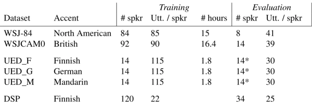
5.1 Speech corpora . . . 33

5.2 Accented Speech in Training . . . 35

5.3 Neighbours of UED_F speakers . . . 39

5.4 Near Neighbour Tranformations . . . 40

5.5 Neighbour, Accent and Stacked Transformations . . . 42

5.6 Statistical Significance Stacked Transformations . . . 43

5.7 Accent and Stacked Transformations on models trained with foreign ac-cented speech . . . 45

(8)

Symbols and Abbreviations

o(t) Observation vector at timet

µ Mean vector of a multivariate Normal Distribution

Σ Covariance matrix of a multivariate Normal Distribution

ASR Automatic Speech Recognition

CMLLR Constrained Maximum Likelihood Linear Regression CV Cross Validation

DRT Dimensionality Reduction Technique

DSP DSP Speech Corpus, Finnish accented speech corpus recorded at Aalto Universities Digital Signal Processing Course in 2010 and 2011

EM Expectation-Maximization (algorithm) HMM Hidden Markov Model

LM Language Model

LVCSR Large-Vocabulary Continuous Speech Recognition MLED Maximum Likelihood Eigenvoice Decomposition MLLR Maximum Likelihood Linear Regression

PCA Principal Component Analysis SI Speaker Independent

SD Speaker Dependent

UED University of Edinburgh, referring to the foreign accented corpus recorded there

WSJ Wall Street Journal (American English speech corpus)

WSJCAM Wall Street Journal Cambridge (British English speech corpus)

(9)

Introduction

As long as machines have existed, people have been trying to make them understand our language, the spoken word. In comic books and movies often speech can be recognized by computers without a single error. In reality however, computers still have problems recognizing and understanding what we speak to them.

The first speech recognizer was made in 1952 in the Bell Telephone Laboratories (K. Davis, Biddulph, and Balashek 1952), a machine that could recognize spoken digits with high accuracy, between 97 and 99% success rate. Since then a lot has changed. Computers were developed and grew in computation and memory capacity exponentially, with the amount of transistors doubling each two years (Moore’s law). Still, no applications exist that can recognize a broad range of speech, in vastly different environments with such a high accuracy and speed as humans can.

There is also good news. When a lot of speech data is available from a single person, and only the speech of this particular person needs to be recognized, or in case the domain of words spoken is limited, speech recognizers can recognize with very high accuracies. Therefore, a mobile phone can recognize which contact to call when a name is said and automatic telephone services can determine with which customer representative to connect to, when told what the problem is. Also, dictation and transcription services exist but almost all books and articles, including this thesis, are still typed and not dictated.

The main reason why digit recognizers or voice command operated applications work is because of the limited domain of words that need to be recognized. Also, the words can appear in limited combinations, mostly defined by some simple rules. When recognizing full sentences, the number of possible words increases greatly and the grammars are not easily described as a set of rules.

Recognition is even more complicated in cases where also humans have sometimes trouble understanding each other. Voices vastly differ from each other, as do speaking

(10)

Chapter 1. Introduction

styles. When people speak in their own local dialect or people are not native to a language, they are often hard to understand. Still, when it is heard often enough, the dialect or accent will become perfectly understandable.

This thesis tries to find methods of improving recognition by using data of other speakers with similar features. Like it will be easier for a person to understand a foreign accent after hearing multiple persons speaking it, a speech recognizer should be able to take advantage of available data with a foreign accent by training or adapting statistical models that describe this particular accent and utilize this to improve the recognition.

1.1

Goals of this thesis

The goal of this thesis is to research methods to improve the speech recognition results by adapting the recognizer with speech data of speakers other than the target speaker. These speakers could be either selected in supervised (speakers pre-grouped by gender or dialect) or unsupervised (speakers grouped automatically) manner. The findings will be tested on different foreign accent data sets to show whether the methods are generic between accents. Also experiments will be done to measure the influence of the amount of speech data available for adaptation.

The main purpose is to improve adaptation for speakers with only very limited amount of speech data available. This thesis also considers the practical needs for real-world applications, taking into account requirements such as speed and required computational resources.

1.2

Speech Recognition at Aalto University

The Speech Group at Aalto University, where this work was done, is part of the department of Information and Computer Science and is led by Docent Mikko Kurimo.

The group has a long history of speech recognition, especially for the Finnish language. The first PhD thesis in speech recognition was Jalanko (1980), which developed a system for labeling speech, useful in a small vocabulary (1000 words) system. Late 1980’s, a phonetic typewriter was developed (“Workstation-based phonetic typewriter”; Torkkola et al. 1991). Kurimo (1997) applied Self Organizing Maps and Learning Vector Quantization (both developed in the same department) for the training of Mixture Model HMMs.

After that a lot of research has been done on Large Vocabulary Finnish Speech recog-nition. Statistical morph-based large vocabulary speech recognition was introduced in

(11)

V. Siivola et al. (2003) and further developed in Mathias Creutz (2006); Hirsimäki et al. (2006).

The group has developed it’s own Speech Recognizer which is used for research purposes. The focus of research has been mainly on the Finnish Language. Finnish is an agglutinative language, meaning that words can be split easily into smaller parts, named morphemes. The Speech Group has, together with the Natural Language Processing group, made vast advances in developing morphological language models. Besides Finnish these methods also have been applied on Estonian and Turkish (Kurimo, Puurula, et al. 2006).

Currently the group researches on methodologies for many aspects of large vocabulary speech recognition and also speaker adaptation for speech synthesis. One sub group focuses on noise robust speech recognition, in which methods are developed to enable recognition for noisy environments. Another focus area is in acoustic model training and adaptation algorithms, where this thesis belongs to. The other research areas are training and adaptation methods for language modeling and the applications of large vocabulary speech recognition in synthesis, retrieval and translation of speech.

1.3

The EMIME project

This work was funded by the European Community project for Effective Multilingual Interaction in Mobile Environments which had the goal of developing personalized speech to speech translation on a mobile device. The potentials of this project are high, as it would enable people to naturally speak on the phone with each other, even though they don’t speak or understand the language of their conversation partner.

Important part is also the personalization of the speech synthesis. When talking with an elderly women, it is unnatural to hear a voice of a young boy speaking. Or when speaking to a man that is careful with his words, speaking slowly, and a deep voice, it is unnatural to hear a fast speaking voice on a higher tone. A third example is maybe even more important, when we hear Finnish men speaking English, we expect some degree of a Finnish accent in the English speech, which helps us to recognize this person’s voice.

The personalization problem is related to the synthesis part of the application, but can be also translated to speech recognition, where similar models are used. As it is hard to personalize a voice in synthesis, for example with an accent, the equivalent problem in speech recognition is to recognize this particular type of voice.

This thesis focuses on recognizing foreign accented speech, but these methods could later also be applied to synthesis, potentially making to easily create accented synthesized voices and provide rapid speaker adaptation.

(12)

Chapter 2

Components and models in a speech

recognition system

The task of an Automatic Speech Recognition (ASR) system is to automatically transcribe speech to text or commands. ASR systems are for example used in phone services or dictation services. Where in TV-series and movies computers seem to be able to perfectly and instantaneously recognize any speech in any language, in reality the performance in speed and accuracy depends heavily on the conditions, the speaker, the type of speech, and the vocabulary and language used.

For small vocabulary recognition systems, such as digit recognition or command recognition, systems exist that can recognize with a very high accuracy. Therefore, current research is mostly focused on so-called Large-Vocabulary Continuous Speech Recognition (LVCSR) systems that can recognize anything said in a certain language. Also for LVSCR already well-performing recognizers exist, but they are often very sensitive for change in speaker, noise-conditions or differences in speaking style (e.g. dictation vs. free speech). Improving the robustness of recognizers, or enabling recognizers to adapt to new conditions is one of the focus areas of the ASR community (Baker, Deng, Glass, et al. 2009). Another focus is the usage of high volume corpora. Some people try to create enormous well transcribed, high quality corpora, while others try to utilize the enormous amount of speech data available on the Internet. (Baker, Deng, Khudanpur, et al. 2007).

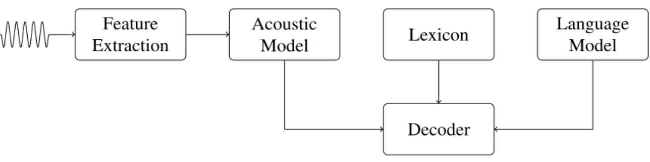
State-of-the-art ASR recognition systems consist out of four separate models. First, Feature Extraction transforms a speech signal into sequential data vectors, called feature vectors. The feature vectors are matched with their corresponding sounds in the Acoustic Model. The Acoustic Model describes for every sound in the language, how the feature vectors are distributed. These sounds often generally match with the phones used in a phonetic alphabet. Words are described in the Lexicon, which is a list of all different

(13)

Feature Extraction Acoustic Model Lexicon Language Model Decoder

Figure 2.1: The main components of an ASR system

pronunciations for each word that must be recognized by the system. The last part is the language model that describes how the language that is recognized is structured. In English for example, after the word ‘red’, it is possible that the word ‘wine’ is used. However, after the word ‘wine’, the word ‘red’ wouldn’t be on the right place in the sentence. The Language Model describes constraints of the language, to make recognition of normal sentences possible. These four different models are shown in Figure 2.1. The fifth component of the ASR system is the decoder. The decoder finds the sequence of words that fit the best in the combination of the acoustic and language model, given an input audio signal.

In the next sections, all the four different models are described. After that the decoding with the whole system is explained. The last part is the metrics used for evaluation of ASR systems. Because this thesis focuses on improving the acoustic model for foreign accented speech, the acoustic model will be described most extensively.

2.1

Speech Signal

Sounds, including speech signals, are transported as pressure differences in the air. The pressure changes differ in frequency and these frequencies are perceived by the human ear as tones and their amplitude corresponds with loudness. To digitize the sounds a microphone records a high number of samples each second of the pressure differences. The number of samples per second is called the sample rate and the number of bits precision used to record the pressure differences is called the bit-size. Figure 2.2 shows an example of a sound signal for the words “speech recognition”. Here a sample rate of 16 kHz and a precision of 16 bits is used for the accuracy of each frame (meaning each frames can have 216=65536 different values).

(14)

Chapter 2. Components and models in a speech recognition system

/s/ /p/ /iy/ /ch/ /r//eh/ /k/ /ah/ /g/ /n/ /ih/ /sh/ /ah/ /n/ Figure 2.2: The sound signal for the words “speech recognition”

2.2

Feature Extraction

The digital speech signal is not immediately useful for ASR. As speech is formed by the frequencies of the sound, the speech should be transformed from the time domain to the frequency domain. Because sound is a mixture of signals with different frequencies, the signal in the frequency domain will be multidimensional, with every dimension describing the amplitude of the components in some frequency range.

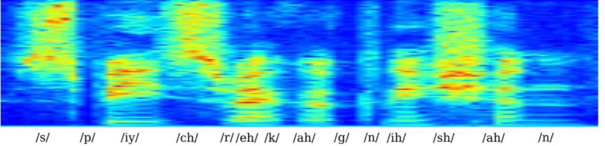
The most common way of extracting frequencies are Fourier Transforms and in this case, because we have digitized data, the Discrete Fourier Transform (DFT) (Cooley, Lewis, and Welch 1969). As our signal is quasi-stationary (O’Shaughnessy 1987, p. 40), i.e. stationary over a short time span, we calculate the transform over short, overlapping time windows, which is also called the Short Time Fourier Transform (STFT). To smooth the overlap between windows, Hamming windows are used. Typically the window size used in ASR is between 20 and 25 milliseconds. A common overlap for the windows is 10 ms. This results in 100-125 frames per second, with each frame being a large vector of Fourier coefficients. In Figure 2.3 the STFT spectrum (the energies of different frequencies) is shown for the same data as used in Figure 2.2. Here a window of 25 ms is used.

/s/ /p/ /iy/ /ch/ /r//eh/ /k/ /ah/ /g/ /n/ /ih/ /sh/ /ah/ /n/ Figure 2.3: STFT spectrum for the words “speech recognition”

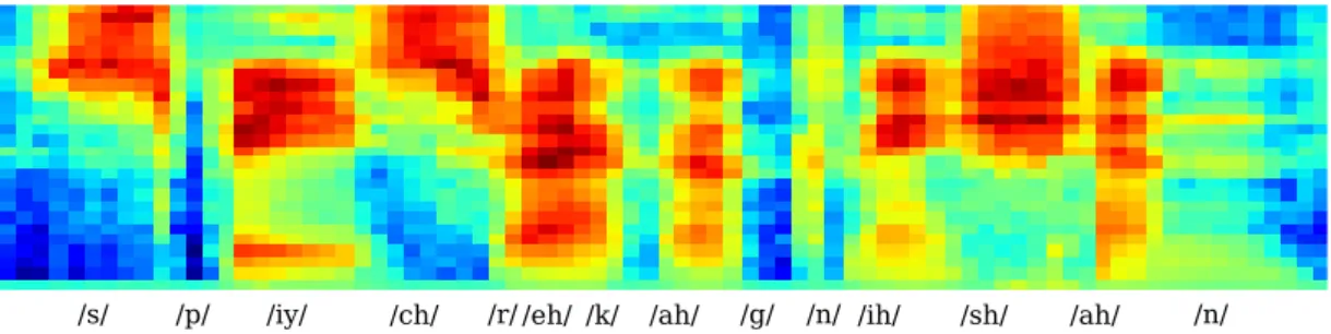
Not all frequencies are equally important when recognizing speech. Therefore, also the human ear is more sensitive to certain frequencies. Inspired by this detail the mel-scale was developed by Stevens, Volkmann, and Newman (1937) to model the human ear. A

(15)

scale filter bank can be used to transform a frequency spectrum into a mel-scale spectrum. The mel filterbank defines a number of ‘bins’, that are equally spaced on the mel-scale. The signal is divided over these bins, and as the bins for the most important frequencies are smaller, these frequencies are amplified. On the frequency scale, triangular windows are used to assign the frequencies. An example of the windows is shown in Figure 2.4. Commonly between 24 and 40 bins are used as it utilizes the effect of the mel-filter bank, but also reduces the dimensionality of the data. The formulas are summarized in X. Huang, Acero, and Hon (2001, pp. 316–318). The resulting mel-spectrum is shown in Figure 2.5.

Frequency

Magnitude

Figure 2.4: Melfilterbank with 26 components

/s/ /p/ /iy/ /ch/ /r//eh/ /k/ /ah/ /g/ /n/ /ih/ /sh/ /ah/ /n/ Figure 2.5: Mel spectrum for the words “speech recognition”

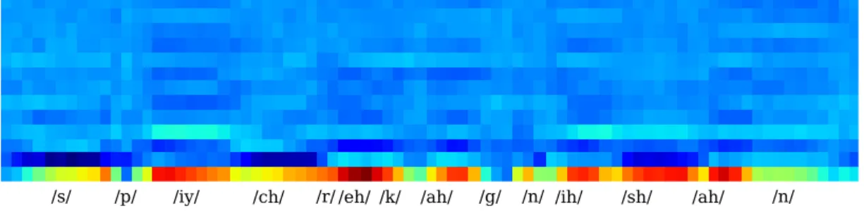
It is desirable for the acoustic model to operate on lower-dimensional, de-correlated fea-tures. Thus, the logarithm is taken of the features and then the Discrete Cosine Transform (DCT) is used to transform the mel spectrum into the mel cepstrum. As a consequence the energy will be collected in the lower indices with the first component being only the energy. Often the number of final components is thirteen. In Figure 2.6 the result after the DCT is shown. Visually the different phonetic units are not as easily recognizable as with the spectrum, but for the acoustic models these vectors are much better.

These 13-dimension vectors are called the Mel-Frequency Cepstral Coefficients (MFCC). MFCC’s were first used in Mermelstein and S. Davis (1980) for speech recognition. Cur-rently, often the first and second derivatives are added to retain more temporal information,

(16)

/s/ /p/ /iy/ /ch/ /r//eh/ /k/ /ah/ /g/ /n/ /ih/ /sh/ /ah/ /n/ Figure 2.6: Mel cepstrum for the words “speech recognition”

improving recognition performance (Furui 1986), which makes the feature vectors 39-dimensional.

2.2.1

Feature level normalization

Multiple methods exist to enhance the robustness of the features for different environments, such as noise on the background or type of microphone. A basic method is Cepstral Mean Subtraction (CMS), which is used for all experiments done in this thesis. CMS is a simple technique that normalizes for each utterance the features. As a result, the conditions that are constant in an utterance, such as microphone type, are normalized away (Atal 1974).

2.3

Acoustic Model

As there are many options for choosing the feature extraction method, multiple different acoustic models are possible. Most of the current state of the art systems use Hidden Markov Models (HMM) with Gaussian Mixture Model (GMM) emission distributions.

This section will first define how phonemes are selected and then how their acoustics can be modeled with GMMs and their temporal properties with HMMs.

2.3.1

Phoneme set

An important decision for the acoustic model is which phonetic alphabet to use. Unlike for example Finnish, the English language does not always have a straight translation between a letter in the normal alphabet and it’s pronunciation. For example the words toy and cow both have an ’o’ as middle letter, still the pronunciation is completely different. Further a word can have different pronunciations depending on its meaning or the dialect or accent of the speaker.

(17)

Multiple phonetic alphabets have been developed that can be used to transcribe a word into phonemes that have a direct translation with a pronounced sound. The most known one is the phonetic alphabet of the International Phonetic Association (IPA1) (Ladefoged 1990) which describes all sounds used by languages all over the world. Any single language will only use a subset of these sounds. Another commonly used alphabet for English is the ARPABET, which is used for the recognizers in this thesis. The phonemes and example words for ARPABET are shown in Table 2.1, where the first section is the original set published by the Advanced Research Projects Agency (ARPA, nowadays DARPA) and the second section the extension made for British English. For clarity, to distinguish normal letters from pronunciation phonemes, the phonemes are enclosed by ‘/’ signs.

When a phoneme set is used, there must exist a lexicon for the words to be recognized. The lexicon is a list of words in a language and all their possible phonetic transcriptions. Most of the time not all words in a language are represented in the lexicon, but at least all words that are used in the training data and language model. In a lexicon a single word can have different phoneme transcriptions, to illustrate, the word ‘the‘ could be pronounced as ‘thee’ or ‘thuh’. Additionally, different words could share the same phoneme transcription

such as ‘two’ and ‘too’. The lexicons used in this thesis are described in Section 5.1.2.

Triphones

Often the pronunciation of a phoneme is affected by the phonemes pronounced before and after it. To model this difference, a model could be created for every different context a phoneme appears in. The phoneme ‘a’ could expanded to all different contexts of ‘a’, e.g. ‘t-a+s’ which means an ‘a’ preceded by a ‘t’ and succeeded by an ‘s’. If we would have

38 different phonemes plus a silence phoneme (like in the ARPABET), this would mean 39·39=1521 models would be used for each phoneme.

Triphones are used to get even more accurate and precise acoustic models. The disadvantage is the size increase of the model and the need for more calculations when decoding. The middle way is to have different emission distributions for often used triphones and shared emission distributions for less used triphones. The process of tying these Gaussians is described in Section 2.3.4. In the next sections the word phoneme is used for both single phonemes (monophones) and triphones.

1_{The acronym IPA is often used as an abbreviation for International Phonetic Alphabet, even though that} is technically incorrect

(18)

Phoneme Example Translation /AA/ odd AA D /AE/ at AE T /AH/ hut HH AH T /AO/ ought AO T /AW/ cow K AW /AY/ hide HH AY D /B/ be B IY /CH/ cheese CH IY Z /D/ dee D IY /DH/ thee DH IY /EH/ Ed EH D /ER/ hurt HH ER T /EY/ ate EY T /F/ fee F IY /G/ green G R IY N /HH/ he HH IY /IH/ it IH T /IY/ eat IY T /JH/ gee JH IY /K/ key K IY /L/ lee L IY /M/ me M IY /N/ knee N IY /NG/ ping P IH NG /OW/ oat OW T /OY/ toy T OY /P/ pee P IY /R/ read R IY D /S/ sea S IY /SH/ she SH IY /T/ tea T IY /TH/ theta TH EY T AH /UH/ hood HH UH D /UW/ two T UW /V/ vee V IY /W/ we W IY /Y/ yield Y IY L D /Z/ zee Z IY /ZH/ seizure S IY ZH ER /AX/ aboard AX B AO D /EA/ aero EA R OW /IA/ fear F IA R /OH/ bombs B OH M Z /UA/ bourne B UA N

Table 2.1: The ARPABET phonemes, with in the second section the phonemes exclusively used for British English.

(19)

2.3.2

Gaussian Mixture Models

In the acoustic model, sounds are modeled with Gaussian Mixture Models (GMM). Each phoneme could have a single GMM, but when Hidden Markov Models (HMM) are used, even phonemes are split into separate parts, e.g. sub phones, that all have their own GMM. A GMM is a weighted sum of one or more Multivariate Gaussian distributions. So for a GMM withK components, the distribution is defined as

X ∼ K

∑

k

φkN (µk,Σk)

with µ_k and Σk being the mean vector and covariance matrix of Gaussiank and φk

being the weight of Gaussiank.

If there would be no temporal structure between frames, and training a sufficiently different model for each acoustic sound could be done, it would enable recognizing for each the frame the most likely phoneme. In reality, however, sounds are so similar that strict separation of sounds is not possible. Besides, a frame-wise phoneme classification is still not easily transferred to transcription in words as one misclassified frame could mess up the recognition and a single sound could easily have different labellings. The main problem is the lack of temporal information stored in a single GMM. Still, they are very useful, and in fact used as the basic building blocks of more advanced models, e.g. HMMs as described in the next section.

Parameters of a GMM can be trained with the Expectation Maximization (EM) algo-rithm using the Maximum Likelihood criterion (Bilmes 1997). The EM procedure is an iterative procedure that works in two steps. One step is assign each feature to a mixture component and the second step updates the mixture weights, means and variances. Every iteration of the procedure guarantees an increase in likelihood of the model. EM with HMMs and GMMs is explained in Section 2.3.3.

2.3.3

Modeling temporal structures with Hidden Markov Models

To take into account temporal structure in the feature vectors, Hidden Markov Models (HMM) can be used. HMMs are an extension of a Markov chain.

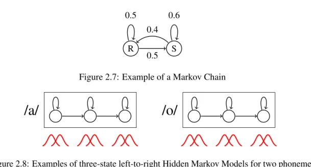
A Markov chain is a network of states. Every time moment the system will be in one state. The probability of being in a state at a certain time, is only dependent on the state of the previous time frame. A demonstration of a Markov chain with two states; Rain and Sunshine is shown in Figure 2.7. Between the states are arcs with the transition probabilities. States can have self-loops, meaning that a state can appear several consecutive times. In

(20)

Chapter 2. Components and models in a speech recognition system R 0.5 S 0.6 0.5 0.4

Figure 2.7: Example of a Markov Chain

/a/

/o/

Figure 2.8: Examples of three-state left-to-right Hidden Markov Models for two phonemes the example, when on day one it rains, the probability for it to be raining on day two is calculated by simply taking the transition probability from Rain to Rain, which is 0.5. The probability for it to be raining on day three is still easy, but involves summing up the options that there is sunshine on day two and raining on day three or raining on both days. The probability for the first is 0.5·0.4=0.2 and for the second 0.5·0.5=0.25. The total probability is 0.45 for it to be raining on day three, if it rains on day one.

In formulas, it is written that the variableX (which can be rain or sunshine) at timet is only dependent onX of timet−1 :

P(X_t|X₁, . . . ,X_t₋₁) =P(X_t |X_t₋₁)

Where in a Markov model the state can be observed, in HMM’s the real states are not discretely observed, such as the Rain or the Sunshine, instead they have an ‘emission distribution’. The Sunshine and Rain example can be in a different country, and the only data available is is the humidity percentage. Even though the Sunshine and Rain can’t be observed, from the humidity can be inferred what most likely is the case.

For speech this means that the hidden state is the label of an acoustic sound, a phone or a sub phone and emission distribution is a distribution of the realizations of this speech, the feature vectors. From a feature vector, not directly can be observed what the state is that generated it, but the probability it is emitted from any state can be calculated.

In Figure 2.8 two HMM’s for two different vowels is shown. Each vowel is separated in a begin, middle and end part, a so called three-state HMM. The emission distributions are GMMs which were introduced in the previous section.

(21)

The notations for a HMM are as follows. The HMM has two kinds of parameters, the transition probabilities between states and the emission probabilities for each state. These parameters together are denoted asλ. Now there are two sequences, a sequence of observationsO= (o₁, . . . ,o_T), the feature vectors, andQ= (Q₁, . . . ,Q_T), the sequence of hidden states that has produced (and ‘explains’) this observations. For recognition, the model is used in such way, that the sequenceQwith the highest probabilityP(Q|λ,O)is found.

For the purposes of ASR, left-to-right models are used, meaning that all states are ordered and no arcs exist from a state to any of it’s previous states. Logically, a backward arc in a phoneme HMM would mean that the beginning of a phoneme is pronounced again after the middle part, practically left-to-right models are used as it is a requirement for computational feasible decoding with the Viterbi algorithm. Rabiner (1989) gives more thorough examples of HMMs in ASR.

Training with Baum-Welch

An HMM can be trained with the Expectation Maximization (EM) algorithm, which in case of an HMM with GMM emission distributions is called the “Baum-Welch” algorithm (Baum et al. 1970). A more introductory explanation is given in Bilmes (1997). The auxiliary function is reasonably simple:

Q(λ,λ0) =

∑

q∈Q

logP(o,q|λ)P(O,q|λ0)

Hereλ0are our current (previously estimated or guessed) parameters of the HMM and λ the new parameters.Qare all possible sequences of lengthT, whereOis the observed data, also of lengthT. The Baum-Welch algorithm increases the value of this function with each iteration, until a maximum is reached.

In the Baum-Welch algorithm, a composite HMM is created. The composite HMM exists out of all HMM’s combined after each other, according to the available transcription. For each time frame of the speech data, the occupation probability for each hidden state of the composite HMM is calculated. When the state occupation probabilities are known, the parameters of the output distributions (µ,Σ) can be re-estimated.

2.3.4

Tying of Gaussians

A large ASR system can have a lot of Gaussians. In case the GMM’s have 16 Gaussians per mixture and a triphone, three-state model with 20 phonemes is used, there would be

(22)

16·3·20·19·19=346560 Gaussians.

A great number of Gaussians has several disadvantages. First, there is not enough data to train every Gaussian and it is unlikely that every triphone occurs so often that 16·3=48 Gaussians could be trained. Some triphones such as ‘t-p-t’ may not occur at all. Secondly, a computationally expensive part of the recognition procedure is the calculation of occupation probabilities for each frame from each Gaussian. Hence, a smaller number of Gaussians would speed up calculations.

Reducing the number of Gaussians can be done by tying similar Gaussians together (Odell 1995; Young, Odell, and Woodland 1994). The similarity can be expressed in a supervised manner, as a list of rules about which phonemes are vowels or consonants, nasal or not nasal, stopping etc. The similarity can also be expressed in an unsupervised way, as a distance measure between Gaussian distributions. The supervised or unsupervised rules are used to build a decision tree. Decision trees are similar to the regression class trees used in adaptation which are described in Section 3.2.1

2.4

Language Model

The language model describes the structure of a language. It tries to prevent the construction of malformed sentences and uses the information of its grammar to rank possible output hypotheses.

The most common language model is the n-gram language model. In an n-gram language model, the likelihood of a word is defined by itsn−1 previous words.

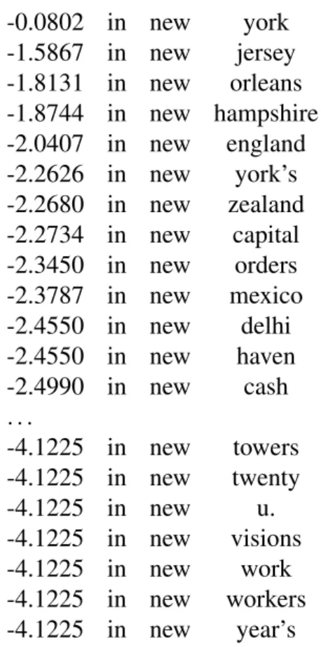
Table 2.2 shows an excerpt from ann-gram model. It shows the log-probability for different words after the sequence ‘in new’. Clearly, in the model ‘in New York’ seems to be the most popular phrase. The phrase ‘in new year’s’ is still likely enough to be in the model, but has a much lower probability than the ‘in New York’ phrase. Unlikely transcriptions are not mentioned at all in the language model to reduce the size and complexity of the model. An extensive explanation ofn-gram language models can be found in Manning (1999, pp. 191-224).

In recognition, the likelihood of different hypothesis will be calculated from the language model and joined with the acoustic probabilities to determine to most probable transcription.

(23)

-0.0802 in new york -1.5867 in new jersey -1.8131 in new orleans -1.8744 in new hampshire -2.0407 in new england -2.2626 in new york’s -2.2680 in new zealand -2.2734 in new capital -2.3450 in new orders -2.3787 in new mexico -2.4550 in new delhi -2.4550 in new haven -2.4990 in new cash . . . -4.1225 in new towers -4.1225 in new twenty -4.1225 in new u. -4.1225 in new visions -4.1225 in new work -4.1225 in new workers -4.1225 in new year’s

Table 2.2: An excerpt from ann-gram language model; the log-probabilities for different words after the sequence ‘in new’.

2.5

Decoding

As shown in Figure 2.1 in the beginning of this chapter, the decoding stage in ASR utilizes all parts of the model. From an utterance that needs to be recognized, the feature vectors are extracted and the probabilities for all states are calculated. The decoder builds a search network and generates a number of hypotheses. The hypotheses are ranked according to their joint acoustic and language model probability.

This decoding is done with the Viterbi algorithm which was proposed in Viterbi (1967) and explained in Forney (1973). In the Viterbi algorithm sequence of phonemes can be found that best describes an sequence of observation vectors from a HMM. The probabilities of the language model are taken jointly with the acoustic probabilities to select the path that is both good according to the acoustic and according to the language model.

(24)

2.6

ASR evaluation

The evaluation of an ASR system can be done in multiple ways. Some measures can be done to describe the fit of the acoustic and language models, or the whole system can be evaluated at once. For an English LVCSR, the latter is often done with help of the Word Error Rate (WER) of a recognition run. To detect real improvements in the WER, statistical significance tests are used.

2.6.1

Recognition run

Evaluating the whole performance of an ASR system must not use any data that is used in the training of the ASR system. Therefore, the recognition utterances must be from speakers who were not used in the development of the acoustic model and the recognition sentences must be different than the ones used in any training files. Most corpora have predefined sets for training and evaluation, sometimes even a separate development set, and if possible these sets should be adhered to, to make comparisons between different studies possible.

2.6.2

Cross validation

A common technique used in Machine Learning, but less in Speech Recognition is the use of cross validation (CV) (Kohavi 1995). This technique splits the data set in toN parts, and trains and evaluates the models with different subsets of the data. For example, N recognitions are done where the evaluation data is one part, and the otherN−1 parts are used for training.

The advantage of this technique is that the data is used more efficiently, as there is no need to excluded one big evaluation set from training. On the other hand, more models have to be trained and evaluated, often resulting in more need of computing resources. Consequently, ASR not often uses CV. In many cases, the corpora are so big that only a small part of the data needs to be used for evaluation. Furthermore, training and evaluation of ASR systems are computationally expensive, making CV unattractive. Still, in this thesis CV is used because the bilingual datasets do not have enough different speakers available that there would be enough training data left if a subset of them would be set apart for evaluation.

(25)

2.6.3

Word Error Rate

For evaluation of the whole ASR system, the Word Error Rate (WER) can be calculated by comparing the recognized text and the real transcription of the recognition data. The error measure is the minimum number of steps to get from the recognized text to the transcription, where a step is an insertion, deletion, or substitution of a single word. The number of steps is taken as a percentage of the number of words in the reference transcription to calculate the error percentage. In principle it is even possible to get a higher error than 100%, when the length of inserted texts exceed the length of the reference transcription.

2.6.4

Statistical Significance Testing

The WER is a good measure to evaluate different recognition techniques or models. Nevertheless, when comparing two methods it must be taken into account that there are other factors than the quality of the technique or the model that can play a role in the final result. Often there is a factor of randomness and chance involved in such complicated model.

Statistical significance tests are used to evaluate whether two results are significantly different. In case the difference is not significant, the better result could be just the result of chance.

The common way of comparing recognition results are matched-pair tests, as advised in Gillick and Cox (1989). In this work, we use the Wilcoxon signed-rank test. The Wilcoxon signed-rank test determines for how many of the utterances, one model performs better than the other. In case for all utterances the result improves, it is definitely significant. If however for almost half of the utterances the result degrades, and for the other big half improves, the average will be still better, but the result is not significant.

(26)

Chapter 3

Adaptation

A speech recognizer can come across a wide variety of utterances. Speakers can be different, noise levels can vary and the topic spoken about can range from the weather to rocket science.

Often a model is trained for a certain type of condition, such as a specific speaker, a certain amount of noise or a particular speaking style. Training models, however, for all different conditions is unfeasible, especially, because there are often no samples available in advance of the exact conditions of the utterances that need to be recognized. To overcome this problem, a model can be adapted to a specific condition. Common adaptations are noise adaptation (Compernolle 1989), speaker adaptation and language adaptation (Bacchiani and Roark 2003). The adaptations in this work are about speaker adaptations, adaptations that account for the variety in speech between different persons. Section 3.1 looks into the differences between different types of models, speaker independent or speaker dependent, and in Section 3.2 speaker adaptation is explained. Section 3.3 reviews different methods for adapting to (foreign) accents.

3.1

Speaker-Independent and Speaker-Dependent systems

There are two different kinds of ASR systems. The first category of systems are Speaker-Dependent (SD) systems, which are able to recognize a single speaker. SD models are trained with speech data from this single speaker, to be able to later very well recognize this single speaker. Except for the advantage that a very high performance can be achieved, there are a lot of drawbacks to this approach. A speaker that wants to be recognized must first speak training sentences, that are transcribed. Depending on the desired accuracy, several hours of speech are needed. For normal end-users this is most of the time not feasible, taking simply too much time and costing too much resources for storage and

(27)

transcription of files.

The second category of models are Speaker-Independent (SI) models. SI models recognize most speakers reasonably well, but do not excel for any particular speaker. SI models are obtained by training the model with speech collected from a variety of different speakers. In this way the model captures the variety of pronunciation possibilities, even enabling the model to recognize new speakers whose data was not used in training. Compared to SD models, the advantages are remarkable. No training data is needed when a new voice is to be recognized, which makes it easy for recognizers to start recognizing new speakers. In addition, a moderate amount of transcribed training data from multiple speakers is already commonly available and only one model needs to be stored for all speakers. The drawback is the reduced accuracy compared to a SD model.

3.2

Speaker Adaptation methods

Speaker Adaptation tries to find ways to transform, or adapt a Speaker-Independent model to a Speaker-Dependent model, with the help of only a very little, possibly not transcribed, training (adaptation) data. Speaker Adaptation enables to get high accuracy results like in an SD model, without the drawbacks for recording, computation and storage.

As the difference between speakers is often in the acoustic domain, the parameters that are of interest to be adapted are the parameters of the emission distributions, the means and variances of the Gaussians in the GMMs. Even though there could be also optimal values for the transition parameters of the HMMs, these only give relatively small improvements and are hard to calculate with a limited amount of data. Further, adaptation in the language model could be done for single speakers, but a lot more sentences are needed than for acoustic model adaptation. Therefore, language model adaptation is often done topic wise.

Woodland (2001) defines three classes of speaker adaptation techniques; linear regres-sion techniques, maximum a posteriori techniques, and eigenvoice or clustering techniques. Linear Regression techniques are methods such as Maximum Likelihood Linear Re-gression (MLLR) and Constrained Maximum Likelihood Linear ReRe-gression (CMLLR). These techniques perform a linear transformation on the parameters of the Gaussian mod-els. MLLR and CMLLR are the most common used adaptation techniques. CMLLR is explained in later sections as it is heavily used in the experiments.

Just as in other machine learning applications, instead of Maximum Likelihood, also Maximum a Posteriori (MAP) adaptation can be adopted. In MAP adaptation, the SI model is used as prior and observations of features are used to estimate a posterior distribution (Gauvain and C.-H. Lee 1994). One problem is that for a Gaussian to be updated with MAP,

(28)

Chapter 3. Adaptation

it must be observed in the adaptation data. As a lot of sentences are needed to observe enough data for all Gaussians, more adaptation data is needed for MAP techniques than for example for linear regression techniques. If a lot of data is available MAP will likely perform better than linear regression. Because of the need of much adaptation data, MAP is used less often than linear regression methods.

The third class of adaptation methods are the eigenvoice and clustering techniques (Gales 2000; Kuhn, Nguyen, et al. 1998), which create a space of voices, with every voice being represented as a mixture of base voices. For a new person, maximum likelihood methods can estimate new parameters. In this thesis eigenvoice methods are not used as adaptation method, but as clustering technique and are described more detailed in Section 3.2.2

3.2.1

Linear Regression Methods

Maximum Likelihood Linear Regression

Maximum Likelihood Linear Regression (MLLR) is a method proposed in Gales and Woodland (1996); Leggetter and Woodland (1995), and is a method for doing a linear transform on the mean and variance parameters of the Gaussian distributions in such way that the likelihood of the adaptation data is maximized.

With MLLR, the mean and covariance matrices of the multivariate Gaussians are transformed with different transforms. The mean µ is transformed with matrix Aand vectorbto form the adapted mean ˆµ with

ˆ

µ =Aµ+b

The variance transform is a bit more complicated. From the covariance matrixΣthe

inverse Choleski factorBis derived, to be transformed with the transformation matrixH. The new covariance matrix ˆΣis

ˆ

Σ=BTHB

Constrained MLLR

In contrast to normal MLLR, Constrained MLLR transforms the means and variances of the Gaussian distributions with the same transformation matrix (Digalakis, Rtischev, and Neumeyer 1995; Gales 1998).

(29)

The new transformation matrices are: ˆ

µ =A−1µ+b ˆ

Σ=A−1ΣA−1T

Because often diagonal covariance matrices are used, it is favorable to preserve them as it makes computation of likelihoods easier. With CMLLR however, the covariances are always transformed into full matrices. To circumvent this the feature vectors can be transformed instead, before any likelihood calculations are done. Instead of the above equations, the feature transform becomes now

ˆ

o(t) =Ao(t)−b

Regression Class Trees

Normally in CMLLR and MLLR methods, all distributions are transformed with the same transform, though, this does not have to be the case. MLLR and CMLLR could also be applied to all Gaussians separately. Although it sounds appealing, some complications arise. For 39-dimensional distributions (as common for MFCC vectors), at least a few hundred frames must be used for each Gaussian to give a robust transform that generalizes to new speech. It is unfeasible to collect that much adaptation data, especially because some Gaussians are so rare that they are used only very few times, even in training.

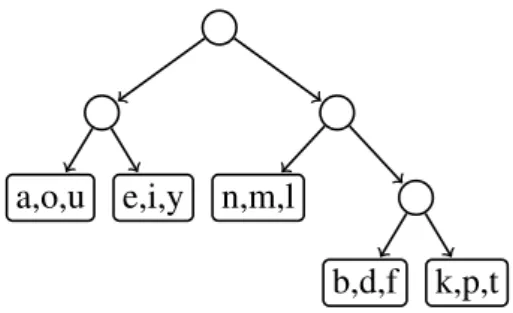
An alternative approach is to group Gaussians together in so-called Regression Class Tree (Gales 1996). All Gaussians will be assigned to exactly one Regression Class, and all Gaussians in the same class are using the same transformation. An example of a Regression Class Tree is given in Figure 3.1. A Regression Class Tree is a binary tree, with only the leaf nodes containing objects. The objects could be Gaussians, or groups of Gaussians; for example all the Gaussians belonging to one phoneme or all Gaussians belonging to one mixture. In the following text the word Gaussian is used, but the procedures are the same for groups of Gaussians.

The Regression Class Tree creation procedure is as follows. First for all Gaussians, the statistics are collected, specifically, by assigning each frame in the training data to the best matching Gaussian. Then all the Gaussians are collected in the root node and an iterative procedure starts. The node with the biggest occupation is split into two siblings. Splitting a node happens with thek-means algorithm (k=2), where the Kullbach-Leibler divergence acts as distance measure between Gaussians. The splitting results in two groups of Gaussians, with the Gaussians in a single group being similar to each other. When the

(30)

Chapter 3. Adaptation k,p,t b,d,f n,m,l e,i,y a,o,u

Figure 3.1: Regression Class Tree with phonemes as unit

number of leaf nodes is equal to a predefined number, or when there are no nodes anymore that can be split, the algorithm terminates.

Applying the Regression Class Tree in adaptation works as follows. In (C)MLLR for each adaptation matrix statistics are collected, which will be used for calculating the matrix. Instead of collecting the statistics for the whole model, as would be done when adapting with only one matrix, the statistics are collected separately for each leaf node. When all statistics are collected each leaf node is evaluated whether it has enough statistics. Having enough statistics depends on available utterances that contain frames emitted by the Gaussians in the leaf node. The amount of statistics required is approximately 1000-4000 frames but depends on the model and type of adaptation trained.

If a leaf node does not contain enough statistics, its statistics are merged with the statistics of its sibling. Going back to Figure 3.1, if the node ‘b,d,f’ does not contain enough statistics, the statistics of nodes ‘b,d,f’ and ‘k,p,t’ are merged together to a new node ‘b,d,f,k,p,t’. This procedure repeats itself until all leaf nodes have enough statistics or only the root node is left over. Now for each leaf node an adaptation matrix is calculated according to the normal procedures. When storing the adaptation matrix, also the Gaussians that are applicable for the matrix must be stored in order to know at recognition time what Gaussians to transform with the adaptation matrix.

The size of the tree is not really relevant, as long as it ‘big enough’. The real number of adaptation matrices used only depends on the adaptation data. For normal recognition the number of final adaptation matrices will be quite small.

3.2.2

Eigenvoices

Eigenvoices is an adaptation method, or more precisely a concept of methods, that uses a low dimensional space to describe different speakers. The parameters of a speaker are the weights for a mixture of parameter vectors that construct a recognition model.

Eigenvoices were first proposed in Kuhn, Junqua, et al. (2000); Kuhn, Nguyen, et al.

(31)

(1998). The principle is to train Speaker Dependent models for a number of speakers, with each model being of the same structure and dimensions. The parameters of the models are transformed into a ‘supervector’ for each model. Afterwards, a Dimensionality Reduction Technique (DRT) is applied to find the bases of the eigenvoice space (eigenspace). In principle every DRT would work, but Principal Component Analysis (PCA) (Jolliffe 2002) is the most commonly used technique.

When the eigenspace is created, multiple methods can be used to estimate the eigen-voice parameters for the new speakers. The process is called eigeneigen-voice decomposition and the most common method is Maximum Likelihood Eigenvoice Decompostion (MLED). For both eigenspace creation and eigenvoice decomposition there are a wide range of methods available. For example, instead of a DRT, a maximum likelihood estimation of the eigenspace can be made (Nguyen, Wellekens, and Junqua 1999). Another popular variation is to not train separate SD models, but to use MLLR adapted models directly (Botterweck 2000; K. Chen and H. Wang 2001) or indirectly (N.-C. Wang et al. 2001).

In this work eigenvoices are not applied as adaptation, but the eigenvoice parameters are used to find similar speakers by looking to the similar speakers in the eigenspace. Both eigenspace computation and decomposition are utilized in the original way and are therefore more thoroughly explained in the following sections.

Eigenspace computation with (C)MLLR adapted models

To calculate the bases of the eigenspace, it is the most convenient to train an SI model and transform it with a CMLLR adaptation to get an SD model for each speaker. This removes the need of training a separate model for each speaker.

A super vector is created by combining and ordering all the mean parameters of the model. The ordering is arbitrary but must be the same for all speakers. With PCA the supervectors are reduced to a small number of parameters, typically between 3 and 10.

Because acoustic models with triphones have a enormous amount of mean parameters, making PCA infeasible, in this work only the single phone models are used for the eigenvoice computations. Using single phone models also reduces the computational needs for decomposition.

The eigenvoice parameters of the training speakers can be directly reconstructed by using the scores obtained with PCA. Also an Eigenvoice Decomposition method could be applied on the training data and ideally the resulting eigenvoice parameters will be the same for both methods.

(32)

Maximum Likelihood Eigen Decomposition

Maximum Likelihood Eigen Decomposition (MLED) finds the eigenvoice parameters that maximize the likelihood of the evaluation data (Kuhn, Junqua, et al. 2000; Kuhn, Nguyen, et al. 1998), by applying the Expectation Maximization (EM) algorithm. As common in EM, an auxiliary functionQ(λ,λˆ)is defined, in this case

Q(λ,λˆ) =−1

2P(O|λ)

∑

_s

∑

_t γs(t)f(ot,s) withf(o_t,s)being the Gaussian log-likelihoods, here defined as:

f(ot,s) = (nlog(2π) +log|Cs|+h(ot,s))

and

h(ot,s) = (ot−µˆs)TCs−1(ot−µˆs)

wheresis a state,nis the number of features,ot the observation vector at timet,C

(s)−1

m

the inverse covariance in states, ˆµsthe new adapted mean of statesandγs(t)the current

likelihoodL(s|λ,ot). These likelihoods are the occupation probabilities, calculated with

the Baum-Welch algorithm (as explained in chapter 2.3.3). Qcan be minimized analytically, resulting in the closed form

∑

t

∑

s

γs(t)eTsCs−1ot =wT

∑

t

∑

s

γs(t)eTsCs−1es

wheree_s are the eigenbases in statesandware the eigenvoice parameters. This closed form can be easily solved as it has the same number of equations as unknowns.

3.2.3

Supervised and unsupervised adaptation

All mentioned speaker adaptation methods take a number of utterances and their transcrip-tion to estimate the adaptatranscrip-tion. In real world systems however, not always the transcriptranscrip-tion of the adaptation sentences is available.

When the transcriptions are known, for example because the speaker read from a prompt or the utterances are manually transcribed, the adaptation is called supervised. When the transcriptions are not known, the baseline recognizer is used to recognize an initial transcription. This transcription is not perfect, but most adaptation algorithms will still work correctly in estimating a good adaptation with them. After that the recognition is done with adaptation to get the better recognition result. In principle this procedure could

(33)

be even repeated, but often the final result will only improve little and the computational costs are high (the cost another adaptation + recognition run). The latter method is called unsupervised adaptation.

3.2.4

Speaker adaptation in real world recognition scenarios

One of the advantages of speaker adaptation compared with training a speaker dependent model is that it is possible to estimate an adaptation in a short time, possibly while the user is waiting for it. The scenario for a first time user is that a speaker independent model exist, with no knowledge of the speaker that is going to be recognized. The system could now either choose to ask the user for uttering some predefined utterances to do supervised adaptation, or to recognize the first sentences without adaptation and to estimate an unsupervised transform with this initial recognition.

In the second scenario, the user might experience a bad performance in the beginning of the recognition, which only can be improved after a few sentences. These sentences have to be stored until the adaptation is estimated, after which only the adaptation matrix (which only is a few kilobytes) needs to be retained.

Compared to the SD trained model this is a substantial improvement. For the training of an SD model hundreds of sentences are needed, the training takes longer and the storage needs per speaker are megabytes of audio in training phase and hundreds of kilobytes per model.

3.3

Accent Adaptation

Besides techniques for adapting the speech recognition system to a specific target speaker, an ASR system can also be adapted to be suitable for recognizing specific accents or dialects. The most basic solution for recognizing accented speech is to train with either exclusively accented speech or to at least include some accented data for training. The problem with the former is that enough accented data (from the same accent) must be available to train a robust model. Both of these methods have the issue that they need training for every accent that will be encountered in recognition. Often, in real world systems, not every accent can be accounted for in advance.

As with the more generic problem with recognizing speakers whose speech was not included in the training data, adaptation can be used to optimize our model for a particular accent. In contrast to speaker adaptation where some ’standard’ methods such as CMLLR exist, the accent adaptation landscape is more diverse. Dialects can differ in pronunciation,

(34)

grammar and vocabulary, all these three areas have there own adaptation points. The pronunciation and vocabulary differences can be corrected with dictionary adaptation (C. Huang, Chang, et al. 2000; C. Huang, T. Chen, and Chang 2004) or acoustic model adaptation (Z. Wang, Schultz, and Waibel 2003).

For foreign accents also cross-lingual adaptation is a possibility (Aalburg and Hoege 2004; Bartkova and Jouvet 2007; Karhila and Kurimo 2010; Liu and Fung 2000). Instead of using adaptation data from the same language as the one being recognized speech data from another language, commonly the target speakers mother tongue, is used. As an example, bilingual models can be trained or phonemes can be mapped between different languages.

Clarke and Jurafsky (2006) shows that basic acoustic model adaptations have limitations in how far they can reduce error rates, but still good results can be achieved. Off course for foreign accents the level of proficiency in the language greatly changes the possibilities for recognition improvement (Tomokiyo and Waibel 2003).

(35)

Stacked Transformations

Stacked Transformation is a method that uses multiple different sequential CMLLR adap-tations to improve recognition. In first instance it is applied to foreign accented speech, but the method could be transferred to normal recognition and to noise robust recognition as well. The method is also described in Smit and Kurimo (2011) which is a conference paper describing the highlights of this method.

The basic idea is inspired by the fact that an important factor for a bad performance when recognizing foreign accented speech is the mismatch between the acoustic models which are trained on non-accented speech and the real acoustic properties of the foreign accented speech that is recognized. Naturally, it would be possible to train a separate model for recognizing the foreign accented speech, resulting in no, or very little, mismatch.

Unfortunately, big corpora of foreign accented speech are scarce. Often the amount of utterances or the number of speakers is limited, which makes it hard to build a model for the foreign accented speech that is as robust as it could be for native speech. In addition, as model training and storage cost a lot of resources, it would be nice if both native and foreign speakers could be recognized with the same models.

The situation is similar to the need for well performing speaker dependent models as described in Chapter 3.1. To obtain a good SD model, already a good approach exists, like the adaptation of SI models into SD models. Similarly we can use the same techniques to transform an SI model into a Speaker-Independent–Accent-Dependent model. Adaptations need much less data than model training and preserve the robustness of the original model.

Besides Speaker Adaptations and Accent adaptations, other adaptations could be thought out that refine the acoustic model parameters to fit a specific group of speakers, such as speakers with the same gender, or speakers with the same age. Adaptations can even be trained without predefined knowledge about the similarity between speakers, but instead the adaptation groups can be determined automatically.

(36)

Chapter 4. Stacked Transformations

Having different types of adaptations raises the interesting possibility of combining the adaptations for recognition. Is it useful to use first an accent adaptation and after that still a speaker adaptation? These stacks of transformations will be called “Stacked Transformations”.

The following sections will describe the new type of adaptations, the accent adaptation and the near neighbour adaptation and the theory behind stacking these transformation to achieve an even better recognition result.

4.1

Accent Transformations

The first step in creating models that could recognize foreign accented speech well, is to gather some data of people with the same foreign accent. With this data a Speaker-Independent–Accent-Independent (SI-AI) model can be adapted into an Speaker-Independent– Accent-Dependent (SI-AD) model. Because the utterances will contain some common features of the accent, the model will be able to recognize this accent much better. Yet, because multiple different speaker are used, the model will still be able to recognize different speakers even the ones that are not first-timers.

The transformation can be the same as for Speaker Adaptation. A difference is that the transformation can have much more adaptation matrices than the normal amount used for Speaker Adaptation, because of more available data.

In normal CMLLR transformations with Regression Class Trees it is common to have a maximum of tens of adaptation matrices, as not often more data is available to train more. With an accented speech corpora, hundreds of robust adaptations can be trained, making the transformation for each group of Gaussians very detailed and specific.

4.2

Near Neigbour Transformations

Besides using a preselected group (such as people with the same accent, or possibly gender), the closest speakers in a corpus could be used for transforming the model. Obviously a problem of how to determine which speakers are similar to the one that needs to be recognized exists.

As a solution, one method is to determine this with help of the eigenvoice technique, which is described in Section 3.2.2. The idea of using eigenvoices for similarity is not new, as it was previously used in Thyes et al. (2000). An eigenspace can be created with all the data available. The training data can overlap with the speech data used in the training of the model, but also additional data can be used. For all speakers in the training set,

(37)

the eigenvoice parameters can be estimated with help of Maximum Likelihood Eigen Decomposition (MLED).

The eigenvoice parameters are an obvious choice for determining the similarity between two speakers. For measuring the ‘distance’ between two speakers, the euclidean distance criterion can be used .

The procedure for recognizing a new speaker is as follows. A few utterances of the speaker are recognized (or transcribed) and the transcription is used for determining the eigen parameters of the new speaker with MLED. As MLED can work with very little adaptation data, it can be applied already on only a few utterances. The distance between the eigen parameters of the new speaker and all the training speakers can be easily computed and the speakers with the closest distances are elected as neighbours. Adaptation can be done in the same way as done for speaker and accent adaptations.

In real-life systems, the utterance of the new speaker can immediately be used as neighbour data for other speakers. If later another similar speaker needs to be recognized, the just recognized data can be also a candidate for usage in the neighbour transformation.

4.3

Stacked Transformations

Multiple CMLLR transformations can be applied to the same model. Commonly, this is already done with global and tree transformations. The idea of stacked transformations is to use different adaptation levels, all with different detail and using different data sources for the adaptation.

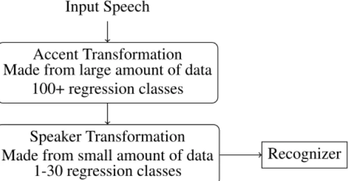
In the case of combining Accent Transformations and speaker adaptations, first a transformation with a big number of adaptation matrices (hundreds) is done to transform the SI-AI model into a SI-AD model. The second transformation will be less detailed and transform the SI-AD model to a Speaker-Dependent (SD) model. The difference between a direct adaptation from an SI to an SD model and the stacked transformation approach is that the knowledge of the characteristics of the accented data is used for both reducing the mismatch and improving the transcription for the Speaker Adaptation. The Stacked Transformation procedure is visualized in Figure 4.1.

Note that the different transformations must have a different level of detail. To recall from Section 3.2.1, a single transformation of a Gaussian is defined by:

ˆ

(38)

Chapter 4. Stacked Transformations

and

ˆ

Σ=BTHB (4.2)

Normally, when two linear transformations are applied, they can be combined to one linear transformation. In that case, the effects of the first transform would be very limited and its effect almost none.

Input Speech Accent Transformation Made from large amount of data

100+ regression classes

Speaker Transformation Made from small amount of data

1-30 regression classes

Recognizer

Figure 4.1: Diagram of the recognition procedure with stacked transformations. The accent transformation is trained with data from multiple speakers with the same accent speakers. The speaker transformation is trained with only data of the target speaker.

4.4

Stacked Transformation computation procedures

In comparison to the scenario described in Section 3.2.4 this section explains how Stacked Transformations could be applied in real life scenarios.

A first distinction that needs to be made is between ‘off-line’ and ‘on-line’ computations. Off-line computations are those that are performed before the data of the target speaker is known or even recorded. In normal recognition with Speaker Independent models, this is only the training of the model. All computations that are done involving the speech of our target speaker are on-line computations.

As we assume that a user would like to have as fast as possible results after inputting the recognition data to the system, the on-line computations need to be reduced to as small amount as possible. On the other hand, for off-line computations no users are waiting for the result, meaning that speed is of less importance.

In unsupervised speaker adaptation there are three steps that need to be performed on-line; recognition of the utterance to provide an initial transcription, estimating a trans-formation with the initial transcription, and after that recognition using adaptation to get the final transcription.

(39)

Even though in stacked transformations more adaptations are used, the same number of steps are needed in the on-line phase as for normal speaker adaptation. An Accent Transformation can be completely calculated off-line before any speaker specific data is known. For a Neighbour Transformation all necessary statistics for making the adaptation can be precomputed, leaving only the discovery of neighbours and the aggregation of statistics for the on-line phase. For the Speaker Transformation all the same steps as outlined in the previous paragraph need to be performed.

4.4.1

Storage requirements

The storage needs for adaptation matrices is only a fraction of the space needed to store a complete ASR model. A typical model used in this work is around 40 megabytes in space and a complete transformation only a few kilobytes.

Again there is only a small need for more storage compared to normal adaptation. In normal adaptation a new transformation is stored for every speaker. In Stacked Transfor-mations only one detailed transformation is stored extra for each accent that is occurred.

(40)

Chapter 5

Experiments

5.1

Datasets and model setup

5.1.1

Speech Corpora

Multiple English Speech Corpora were utilized in the experiments, as shown in Table 5.1. Firstly, the standard Wall Street Journal (WSJ) dataset was used (Paul and Baker 1992). This dataset is used for standard large vocabulary recognitions. All speakers in the WSJ dataset have an American accent. WSJ0 contains 84 training speakers and a evaluation set, the resulting training set is called WSJ-84.

The second corpus is Wall Street Journal Cambridge (WS