Workload-aware Scheduling Techniques for General Purpose Applications on Graphics Processing Units

Graduate Theses and Dissertations

Iowa State University Capstones, Theses and

Dissertations

2017

Workload-aware Scheduling Techniques for

General Purpose Applications on Graphics

Processing Units

Mihir Awatramani

Iowa State University

Follow this and additional works at:

https://lib.dr.iastate.edu/etd

Part of the

Computer Engineering Commons

This Dissertation is brought to you for free and open access by the Iowa State University Capstones, Theses and Dissertations at Iowa State University Digital Repository. It has been accepted for inclusion in Graduate Theses and Dissertations by an authorized administrator of Iowa State University Digital Repository. For more information, please [email protected].

Recommended Citation

Awatramani, Mihir, "Workload-aware Scheduling Techniques for General Purpose Applications on Graphics Processing Units"

(2017).Graduate Theses and Dissertations. 16705.

Workload-aware scheduling techniques for general purpose applications on graphics processing units

by

Mihir Awatramani

A dissertation submitted to the graduate faculty in partial fulfillment of the requirements for the degree of

DOCTOR OF PHILOSOPHY

Major: Computer Engineering

Program of Study Committee: Diane Rover, Co-major Professor Joseph Zambreno, Co-major Professor

Arun Somani Zhao Zhang Glenn Luecke

The student author, whose presentation of the scholarship herein was approved by the program of study committee, is solely responsible for the content of this dissertation. The

Graduate College will ensure this dissertation is globally accessible and will not permit alterations after a degree is conferred.

Iowa State University Ames, Iowa

2017

ii TABLE OF CONTENTS ACKNOWLEDGEMENTS . . . v ABSTRACT . . . vi CHAPTER 1. INTRODUCTION . . . 1 1.1 Motivation . . . 2 1.2 Thesis Contributions . . . 4

1.2.1 Level 1: Intra-core Thread Scheduler . . . 4

1.2.2 Level 2: Inter-core Thread Block Scheduler . . . 5

1.2.3 Level 3: System-wide Kernel Scheduler . . . 6

1.3 Thesis Organization . . . 7

CHAPTER 2. BACKGROUND . . . 8

2.1 The GPGPU Programming Model . . . 8

2.2 Overview of the Hardware Architecture and Scheduling in GPGPU . . . 10

2.2.1 Kernel Scheduler . . . 12

2.2.2 CTA Scheduler . . . 12

2.2.3 Warp Scheduler . . . 14

CHAPTER 3. PHASE-AWARE WARP SCHEDULER . . . 16

3.1 Abstract . . . 16

3.2 Introduction . . . 16

3.3 Phase Behavior in GPGPU Kernels . . . 19

3.3.1 Definition of Kernel Phases . . . 19

3.3.2 Effect of Kernel Phases on Warp Schedulers . . . 21

iii

3.4 Phase Aware Warp Scheduling . . . 26

3.4.1 Scheduling Policy . . . 26

3.4.2 Implementation . . . 27

3.5 Experimental Results . . . 30

3.5.1 Methodology . . . 30

3.5.2 Impact on Performance . . . 31

3.5.3 Impact on Scheduler Idle Time . . . 34

3.5.4 Impact on Functional Unit Load . . . 35

3.5.5 Impact of Intra-Block Tail Effect on Performance . . . 37

3.6 Related Work . . . 38

3.6.1 General Warp Scheduling Techniques . . . 38

3.6.2 Scheduling Techniques to Mitigate Warp Divergence . . . 39

3.6.3 Thread Throttling . . . 40

3.7 Conclusion . . . 42

CHAPTER 4. WORKLOAD AWARE THREAD BLOCK SCHEDULING . 43 4.1 Abstract . . . 43

4.2 Introduction . . . 44

4.3 Perf-Sat: Runtime Detection of Performance Saturation for GPGPU Workloads 45 4.3.1 Motivation . . . 46

4.3.2 Perf-Sat - Underlying Principles and Design Details . . . 51

4.3.3 Experimental Results . . . 54

4.3.4 Related Work . . . 57

4.4 ONAC: Optimal Number of Active Cores Detector for Energy Efficient GPU Computing . . . 59

4.4.1 Effect of Number of Cores on Performance . . . 61

4.4.2 ONAC: Estimation Model and Hardware Implementation . . . 63

4.4.3 Experimental Results . . . 68

4.4.4 Detection Time and its Effect on Power and Energy . . . 72

iv

4.5 Conclusion . . . 76

CHAPTER 5. WORKLOAD AWARE KERNEL SCHEDULING . . . 77

5.1 Abstract . . . 77

5.2 Introduction . . . 77

5.3 Motivation for Concurrent Kernel Execution . . . 80

5.3.1 Compute Benchmark: Add Kernel . . . 81

5.3.2 Memory Benchmark: Stream kernel . . . 83

5.4 Intra-core Concurrent Kernel Execution . . . 84

5.4.1 Kernel to Core Mapping . . . 85

5.4.2 Thread Block Scheduling . . . 86

5.4.3 Handling Kernel Exits . . . 86

5.5 Experimental Results . . . 87

5.5.1 Case Study: Concurrent Execution of Add and Stream . . . 87

5.5.2 Analysis of Runtime Workload Characteristics with Concurrent Kernel Execution . . . 89

5.5.3 Performance Impact with Concurrent Kernel Execution . . . 92

5.5.4 Impact on ALU and Memory Utilization . . . 93

5.6 Related Work . . . 96

CHAPTER 6. CONCLUSION . . . 99

v

ACKNOWLEDGEMENTS

I would like to express my deepest gratitude to those who guided and supported me through the years of my doctoral research. First and foremost, I would like to thank Dr. Diane Rover and Dr. Joseph Zambreno. Putting their faith in me gave me the courage and inspiration that I greatly needed in the initial years of my graduate career. Throughout the course of my graduate studies, their continued patience, guidance and encouragement gave me the support I required to persevere through my doctoral research.

I would also like to thank my committee members, Dr. Zhao Zhang, Dr. Arun Somani and Dr. Glenn Luecke, for taking a keen interest in my work and providing their support through the years. Additionally, I would like to thank Dr. Zhao Zhang, Dr. Phillip Jones and Dr. Joseph Zambreno for their teachings in advanced computer architecture, and Dr. Diane Rover for her teachings in systems design, which helped ignite my passion for the field and guided me to find the right path in the initial years of my graduate school.

Lastly, I would like to thank my parents, my brother and his family, and my fiance Nikita Chopra. Their continued love, patience, support, and words of encouragement has helped me throughout my graduate education.

vi

ABSTRACT

In the last decade, there has been a wide scale adoption of Graphics Processing Units (GPUs) as a co-processor for accelerating data-parallel general purpose applications. A primary driver of this adoption is that GPUs offer orders of magnitude higher floating point arithmetic throughput and memory bandwidth compared to their CPU counterparts. As GPU architectures are designed as throughput processors, they adopt a manycore architecture with 10 to 100s

of cores, each with multiple vector processing pipelines. A significant amount of the die

area is dedicated to floating point units, at the expense of not having hardware units used for memory latency hiding in conventional CPU architectures. The quintessential technique used for memory latency tolerance is exploiting data-level parallelism in the workload, and interleaving execution of multiple SIMD threads, to overlap the latency of threads waiting on data from memory with computation from other threads.

With each architecture generation, GPU architectures are providing an increasing amount of floating point throughput and memory bandwidth. Alongside, the architectures support an increasing number of simultaneously active threads. We envision that to continue making advancements in GPU computing, workload-aware scheduling techniques are required. In the GPU computing work flow, scheduling is performed at three levels - the system or chip level, the core level and the thread level. The work proposed in the research aims at designing novel workload aware scheduling techniques at each of the three levels of scheduling. We show that GPU computing workloads have significantly varying characteristics, and design techniques that monitor the hardware state to aide at each of the three levels of scheduling. Each technique is implemented in a cycle level GPU architecture simulator, and their effect on performance is analyzed against state of the art scheduling techniques used in GPU architectures.

1

CHAPTER 1. INTRODUCTION

In the last decade, the adoption of Graphics Processing Units (GPUs) for accelerating general purpose applications has grown at a rapid pace [33, 35, 50]. The role of GPUs has shifted from being a co-processor for graphics rendering, to a general purpose accelerator for data-parallel workloads [58, 57]. Three reasons can be identified as primary drivers for this rapid growth.

First, the last decade has seen a tremendous growth in the number of highly data-parallel applications, which typically have high computational throughput requirements. Examples can be found in several domains [74] ranging from computational physics [62, 19], medical sciences [61, 70], molecular dynamics [69, 6], computational biology [65] and big data analytics [26]. Currently, a third of the systems in the top 500 supercomputer list use GPUs as accelerators [4]. A clear indication that the growth of GPU computing in the HPC domain would continue to increase in the near future is, the next three supercomputers funded by the U.S. Department of Energy’s CORAL project employing GPUs [38, 56] or similar many-core architectures [36]. Moreover, with the rise of deep learning, GPU computing is expected to grow into several other domains, like automobiles, robotics and urban development [1].

Secondly, with the end of Denard scaling [17, 11] towards the middle of the last decade, improvements in single processor performance from frequency scaling ceased and CPU processor

architectures shifted from single-core to multi-core designs [18]. However CPU cores are

designed for low latency, and thus adopt an architecture with large caches and speculative out-of-order cores [28]. Their computational throughput does not scale to the demands required for the aforementioned high-throughput applications. On the contrary, as graphics rendering workloads have high computational throughput demands and relatively lower latency requirements, GPU architectures employ a many-core architecture and operate at lower frequencies with a

2

significantly higher number of in-order cores [55]. Consequently GPUs provide a significantly higher throughput and memory bandwidth compared to multi-core CPUs, and serve as a natural fit for high-throughput data-parallel workloads.

Lastly, towards the middle of the last decade, GPU architectures started a shift from fixed-function graphics rendering pipelines to programmable shaders [2]. While initial results of using GPU programmable shaders for data-parallel workloads showed significant speedups [13, 66], their adoption was limited due to the difficulty in programming them. With the development of languages like CUDA [12, 34, 49] and OpenCL [47], GPU computing became more widespread, and continues to grow in adoption. This has led to the emergence of a new parallel computing paradigm for executing general purpose applications on GPUs, referred to as GPGPU.

1.1 Motivation

GPU architectures are designed specifically for high throughput computing. For example, the current state of the NVIDIA GPU, the Volta V100, supports a peak double precision floating point throughput of 7024 GFLOPs and a peak memory bandwidth of 807 GB/s [55]. As a comparison, the state of the art Intel CPU, the Xeon E7 supports a peak double precision floating point throughput of 844 GFLOPs and a peak memory bandwidth of 102 GB/s [28]. To achieve such high computational throughputs, GPUs dedicate a large portion of their die area to cores and arithmetic units. As a trade-off, GPU chips do not include the hardware units which have been traditionally used for latency hiding in CPUs. For example, GPUs use a non-speculative in-order pipeline, do not have branch predictors, and have much smaller caches compared to CPUs. As a consequence, GPU architectures typically have an order of magnitude larger static memory load latencies, with dynamic latencies even larger due to the fact that 10s to 100s of cores are executing in parallel.

The primary mechanism to hide the large memory access latencies in GPUs is to perform massive multithreading in hardware. State of the art GPUs support about two thousand scalar active threads per core, and as high as 80 cores per chip [55]. GPGPU programming models divide the workload into three granularities. Consequently, threads are scheduled via three distinct hardware schedulers, each working independently at a different workload granularity.

3

Each function to be accelerated, is offloaded by the CPU as an independent program referred to

as a kernel. A system-level kernel scheduler dictates the scheduling order of the different

kernels launched by the CPU and maps each kernel to a set of GPU cores. The programming model groups threads of a kernel into an abstraction called called Thread Blocks (TBs). Once

each kernel is assigned its respective core by the kernel-level scheduler, a core-level work

distributor issues TBs from each kernel to the cores it has been mapped to. Lastly, threads in

a thread block are grouped as SIMD units called warps [54] (or wavefronts [47]). Consequently,

on each core, awarp-level scheduler interleaves execution of warps launched on a core and

tries to overlap the latency of warps waiting on long latency operations with computation from other warps.

Efficient scheduling of the SIMD threads in hardware has a direct impact on the performance of GPGPU applications. However, due to the extremely high thread counts, efficient scheduling of these threads is non trivial. Moreover, with more general purpose workloads being offloaded to the GPU for acceleration, workload agnostic scheduling techniques that work well for a subset of applications, might fail for others. The motivation of this research is to develop efficient scheduling techniques by using information regarding the workload being executed, and the architecture runtime state. It is important to note that although the overarching goal of the three schedulers is to increase overall throughput, their individual objectives differ considerably as each of them operates at a different workload abstraction. Consequently, this work aims to develop workload-aware scheduling techniques at each of the three scheduling granularities.

Thesis Statement: Thread scheduling techniques play a pivotal role in GPUs to enable

harnessing the high floating point and memory throughput that the architectures support. In this work, we design efficient hardware scheduling techniques at each of the scheduling granularities

in the GPU architecture. We propose that scheduling techniques should be aware of the workload

characteristics, and the architecture state at runtime to maximize the benefits gained from thread level parallelism. Information about workload characteristics is derived at compile time, and

the architectural state is monitored via hardware counters at runtime. This information is used

4

1.2 Thesis Contributions

GPU computing programming models divide the work offloaded to the GPU into a three level hierarchy. Scheduling is performed by hardware units that operate independently at the three levels. In this section, we describe the specific contributions proposed by this research at each of the three levels of scheduling.

1.2.1 Level 1: Intra-core Thread Scheduler

The primary mechanism to hide memory access latency in GPU architectures is to exploit data parallelism in the workload and overlap latency of memory accesses with computation. The context of all threads launched on each core of the GPU is kept live in the respective core’s register file. This enables the thread-level hardware scheduler on each core, called the warp scheduler, to switch among them with low overhead. This scheduler is pivotal in being able to achieve a throughput which is close to peak, as it largely affects how well the computation and memory latency is overlapped. In this work, we show that the performance of existing state-of-the-art warp schedulers is highly dependent on what we refer to as kernel phase behavior [9]. Specifically, the instruction stream of a GPGPU kernel has blocks of compute instructions separated by long latency operations, which we refer to as phases. We thoroughly analyze phase behavior in GPGPU kernels and demonstrate that performance of state-of-art thread schedulers is affected by characteristics of these phases, which vary significantly across kernels. To this end, we design a compiler assisted warp scheduling policy that is aware of kernel phase behavior. The instruction stream of the kernel is analyzed at compile time and information regarding phases is inserted in program instructions. The hardware warp scheduler on the core uses this information to make scheduling decisions. We demonstrate that the phase-aware warp scheduling policy is more robust to kernel phase behavior compared to the existing state of the art warp schedulers.

5

1.2.2 Level 2: Inter-core Thread Block Scheduler

This scheduler operates at a granularity above the warp scheduler, and is responsible for issuing thread blocks to the GPU cores. The primary goal of the thread block scheduler is to keep each core as occupied as possible, by launching threads until the core resources are exhausted. The rationale is, a higher number of threads would give the warp scheduler on the core more opportunities to overlap memory latency and computation, thus resulting in better performance. Consequently, with each architectural generation, as the peak compute throughput and memory bandwidth supported by GPUs continue to increase, each generation supports an increasing number of warps to increase thread level parallelism. For example, the previous generation NVIDIA Pascal chip, the P100, has a peak FP32 throughput of 4.9 TFLOPs, a peak memory bandwidth of 720 GB/s, and supports concurrent execution of 3584

warps [52]. In comparison, the current generation chip, the V100, supports a peak FP32

throughput of 1.4x, a peak memory bandwidth of 1.2x and supports concurrent execution of 1.4x more warps [55].

While increasing thread level parallelism improves performance of latency-limited workloads, the same is not true if the performance of a workload is throughput-limited. We demonstrate that once a workload reaches its peak achievable memory or compute throughput, increasing number of active threads does not improve performance. Consequently, these kernels can be executed with fewer than maximum number of threads without affecting performance. We refer to the number of warps at which performance of a GPU kernel saturates as the kernel’s optimal thread count. Executing fewer than the maximum threads reduces the hardware resources required by the kernel, and enables opportunities for reducing energy consumption by power-gating the unused resources. In this work, we propose two hardware techniques to detect the optimal thread count of GPU kernels at runtime:

1.2.2.1 Executing optimal number of warps on each core

Increasing the number of warps executing on a core decreases the time spent by a kernel waiting on stalls due to data hazard. At the same time, increasing number of warps might

6

increase the number of pipeline stalls due to hardware resource contention. In this work, we analyze the effect of number of active warps on the breakdown of the warp scheduler activity on each core and demonstrate the above effect [8]. We then propose a hardware mechanism, called Perf-Sat, which monitors the scheduler activity on each core at runtime, and detects the optimal thread count independently at each core. The optimal thread count detected by Perf-Sat is used by the thread block scheduler to limit the number of active thread blocks on each core. Our results show that with a performance loss of less than 1%, Perf-Sat is able to achieve core resource savings of 18.32% on average.

1.2.2.2 Executing the kernel on optimal number of cores

An alternative technique (compared to executing optimal number of threads on each core) is to execute the kernel on fewer than maximum core available on the chip. We demonstrate that for memory-throughput limited kernels, executing the workload on fewer than maximum available cores does not significantly impact performance [79]. At the same time, power gating

the unused cores results in significant energy savings. We then propose ONAC (Optimal

Number of Active Cores detector), a hardware mechanism that detects the optimal number of active cores at runtime. ONAC uses an estimation model inspired by Roofline [76], and estimates the effect of number of active cores on the chip’s average IPC. Our results show that, for memory-intensive kernels, ONAC reduces energy consumption by 20% with negligible impact on performance.

1.2.3 Level 3: System-wide Kernel Scheduler

The kernel level scheduler operates at the third and highest level of scheduling on a GPU

chip. It manages binding of kernels to cores on which they would be executed. In GPU

architectures, concurrently launched kernels are scheduled sequentially unless kernels do not have enough threads to occupy all cores. Moreover, when kernels are scheduled concurrently, they are executed on separate cores. As mentioned in the previous subsection, the number of threads required by a kernel to achieve peak throughput is workload dependent, and throughput saturating workloads can be executed with a lower thread count without affecting performance.

7

Executing fewer than the maximum number of warps supported by an architecture frees hardware resources, and opens up opportunities for multi-tasking. Sharing GPU cores among threads from multiple kernels is a relatively new technique, with its own set of challenges [7]. Most previous works have focused primarily on resource partitioning techniques that determine how many cores should be assigned to each kernel. In this research, we focus on the effect of warp scheduling policies in concurrent kernel scheduling scenarios. We demonstrate that kernels limited by complementing resources (memory bandwidth and floating point throughput) show significant speedups when executed concurrently. Our results show that interference among threads from kernels concurrently executing on GPU cores has a performance overhead that effects the gains achieved from concurrent kernel execution.

1.3 Thesis Organization

The remainder of this thesis is organized as follows: in chapter2, we provide background on

the GPU hardware architecture and programming model. Next, we discuss in detail the three levels of scheduling, namely the intra-core warp scheduler, the inter-core thread block scheduler,

and the system-wide kernel scheduler, in chapters 3, 4, and 5 respectively. Each of the three

chapters are organized as a. A background of current state of the art, b. A discussion of the issues that motivate our work, c. A description of our contributions, followed by an in-depth analysis of the experimental results, and d. A discussion of the related published works at the respective granularity of scheduling. Chapter 7 concludes the thesis by providing a summary of the conclusions, lessons learned and directions for future work.

8

CHAPTER 2. BACKGROUND

In this chapter we provide an overview of the programming model used for General Purpose computing on Graphics Processing Units (GPGPU) and the GPU hardware architecture. Both, the GPGPU programming model and the GPU compute hardware architecture have been described extensively in published literature. Consequently, this chapter provides only a brief introduction of the concepts, with more focus on the scheduling work flow in GPU computing. Further details regarding the GPU hardware architecture can be found in [55, 10, 35, 48, 21, 20, 22]. Further details regarding the concepts related to the GPGPU programming model can be found in [34, 12, 47, 54, 51, 74].

2.1 The GPGPU Programming Model

In GPGPU programming models, the GPU is used as a co-processor to the CPU. Sequential

portions of the application are executed on the CPU (referred to as the host), and parallel

portions of the application are executed on the GPU (referred to as the device). The two

most widely used GPGPU programming languages are OpenCL [47] and CUDA C [54]. To evaluate our work, we used applications written in CUDA C. However, the concepts are directly applicable to applications written in OpenCL as well.

The CUDA programming model provides constructs that expose thread-level parallelism and data-level parallelism to the programmer on top of other high level languages. Several languages are supported, like C, C++, Fortran, Python and Java. In CUDA C, the portion of the program executing on the CPU is written in C, and the language provides interfaces (APIs: Application Programming Interfaces) to the programmer to illustrate GPU related functions. A few examples of the APIs provided are, interfaces to query specifications of the

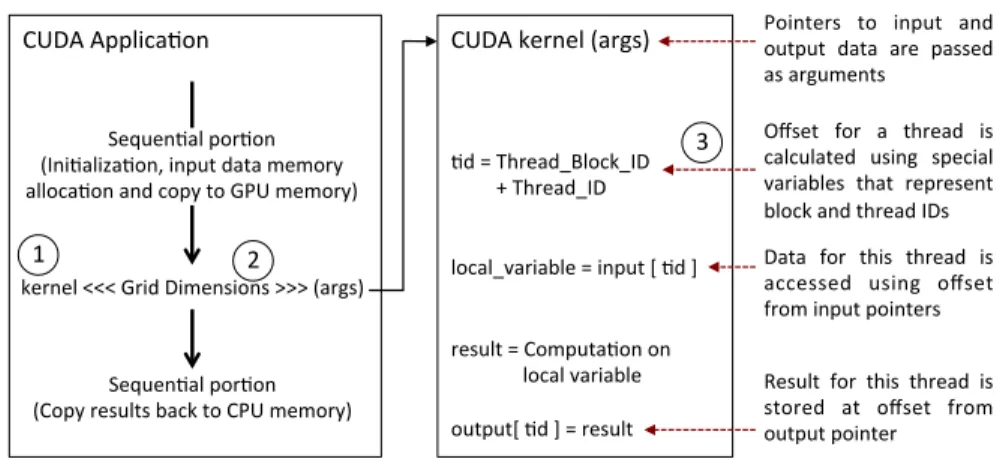
9 Sequen&al)por&on) (Ini&aliza&on,)input)data)memory)) alloca&on)and)copy)to)GPU)memory)) ) CUDA)Applica&on) ) ) kernel)<<<)Grid)Dimensions)>>>)(args)) Sequen&al)por&on) (Copy)results)back)to)CPU)memory)) ) CUDA)kernel)(args)) ) ) ) &d)=)Thread_Block_ID)) )))))))))+)Thread_ID) ) ) local_variable)=)input)[)&d)]) ) ) result)=)Computa&on)on)) ))local)variable) ) output[)&d)])=)result)

Pointers) to) input) and) output) data) are) passed) as)arguments)

Offset) for) a) thread) is) calculated) using) special) variables) that) represent) block)and)thread)IDs) Data) for) this) thread) is) accessed) using) offset) from)input)pointers) Result) for) this) thread) is) stored) at) offset) from) output)pointer)

1) ₂₎

3)

Figure 2.1: Depiction of basic structure of a GPGPU program with one kernel.

GPU (device) on the system (cudaGetDeviceProperties), to allocate/deallocate data on the device (cudaMalloc/cudaFree), to transfer data between the CPU (host) and device memories

(cudaMemcpy), to launch a program (referred to as a kernel) on the device (refer to Fig.2.1),

and APIs that provide synchronization between the host and the device [64, 49, 54] . The application is compiled into a single binary; the sequential portions execute on the CPU, and

GPU related functions are executed by the GPU driver (refer to Fig.2.3).

Fig. 2.1 depicts the basic structure of a CUDA application. As mentioned previously,

portion of the application to be executed on the GPU is written as a separate function, called

a kernel 1. The data which would be operated on by the threads of a kernel is allocated and

copied to GPU memory before the kernel is launched. Similarly, the results are copied back from GPU memory after the kernel finishes. The function launch syntax specifies the total

number of threads that would execute this kernel within the <<< >>>structure (Fig. 2.1 2).

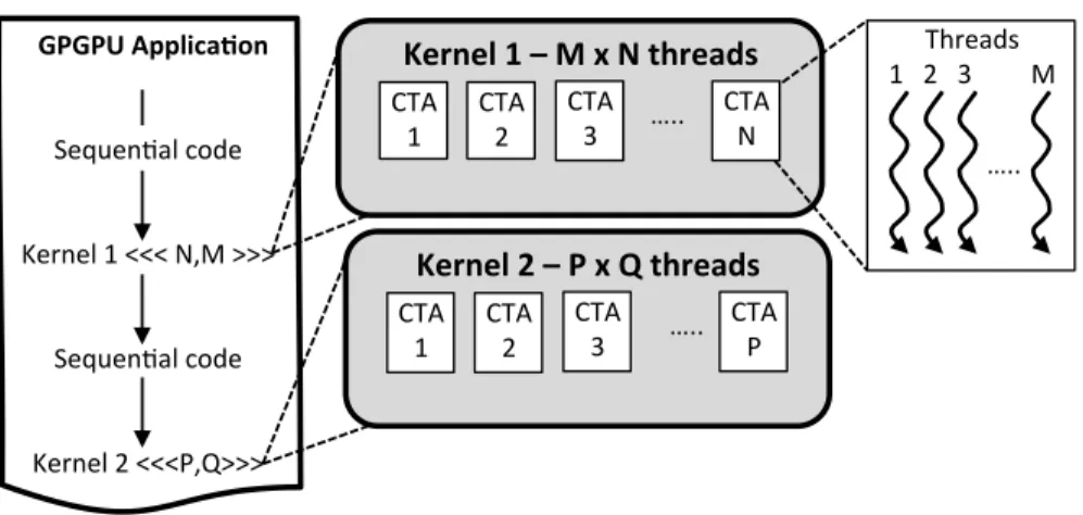
In CUDA, workload for a kernel is described using a two level hierarchy. Fig. 2.2 provides

a depiction of this hierarchy via examples of two CUDA kernel launches. The total number of threads launched for an invocation of the kernel is referred to as a grid. Number of threads in a

grid are described within the<<< >>>structure as(Number of thread blocks, Number of threads

in each thread block). Threads within a grid are divided into groups of threads, called thread

blocks (or CTAs: Cooperative Thread Arrays). The programming model allows for threads within a thread block to use synchronization barriers and share data using an on-chip SRAM.

10 !!GPGPU!Applica+on! ! !!! Sequen'al!code! ! ! Kernel!1!<<<!N,M!>>>! ! ! Sequen'al!code! ! ! Kernel!2!<<<P,Q>>>! PCI!EXPRESS! Kernel!1!–!M!x!N!threads! CTA!!

1! CTA!!2! CTA!!3! !!…..! CTA!!N!

Kernel!2!–!P!x!Q!threads! CTA!!

1! CTA!!2! CTA!!3! !!…..! CTA!!P!

!!…..! Threads! !!!1!!!2!!!3!!!!!!!!!M!

Figure 2.2: Depiction of the thread hierarchy for workload description of a CUDA C kernel.

1 and 2 launch N CTAs of M threads, and P CTAs of Q threads respectively. Each thread executes the kernel instructions on its respective data, resulting in a Single Program Multiple

Data (SPMD) programming model. Figure2.13 depicts how the block and thread identifiers

are used within the kernel to index data specific to a thread from GPU memory. In the next section, we describe how the three level of thread abstractions: the grid, CTAs and threads, are scheduled on the GPU hardware. We encourage the reader to refer to [54, 47] for more details regarding the programing model.

2.2 Overview of the Hardware Architecture and Scheduling in GPGPU

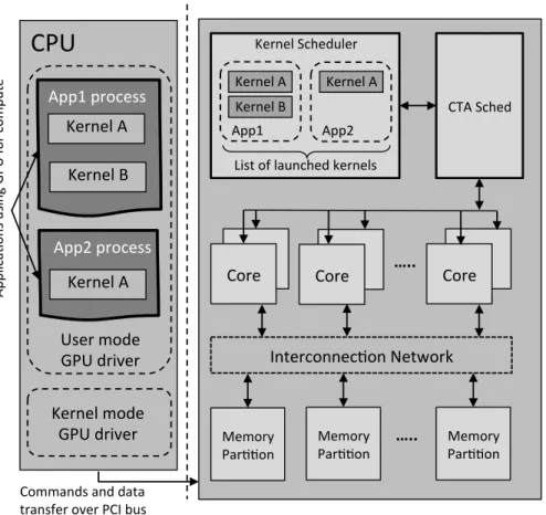
In this section, we provide an overview of the GPU hardware architecture, with a focus on

the flow of scheduling in GPGPU. Fig.2.3 depicts a simplistic block diagram of a single GPU

system, with two GPGPU applications executing on the CPU. Applications 1 and 2 launch two and one kernels respectively. Launching of the kernels, as well as other GPU compute APIs

(refer to Sect. 2.1) are executed via the GPU driver. Data is transfered between the CPU and

GPU using the PCI express or an equivalent bus [52].

At a high level, GPUs have a manycore architecture with several in-order SIMD cores called

SMs, or Streaming Multiprocessors (Fig. 2.3). Each SM consists of several arithmetic vector

execution units (single and double precision floating point units, integer math units, load/store units and special function units used for operations like sine and cosine). Threads launched on a

11

Core!

Core! Core! !…..! Core!

Kernel!A!

CTA!Sched! Kernel!Scheduler!

Interconnec'on!Network!

Memory!

Par''on! Memory!Par''on! !…..! Memory!Par''on!

Kernel!B! App1! Kernel!A! App2! List!of!launched!kernels! Ap pl ic a' on s! us in g! G PU !fo r!c om pu te !

CPU!

Figure 2.3: Block diagram depicting the flow of GPU compute work launch.

GPU core execute instructions on the vector units in Single Instruction Multiple Data (SIMD) fashion. For example, the current HPC chip from NVIDIA, the V100, has 80 SMs, each with four 16-wide SIMD datapaths with 512 bit wide execution units [55]. As context of a all threads launched on the SMs is kept active, each SM has a large register file. Contrary to the CPU architecture, GPUs have a larger register file capacity compared to data cache. For example, the P100 and V100 GPUs have 256 KB of register file per SM, and a total of 14 MB and 20 MB of register file capacity across the chip. In comparison, they have an L2 data cache of 4 MB and 6 MB respectively [52, 55]. Additionally, each SM has a L1 data cache and a high-bandwidth on-chip memory that can be shared by threads from the same thread block. If a memory request misses the L1 data cache, it is routed via the interconnection network to a one of the memory partitions. Each memory partition has a L2 cache bank and a memory controller. GPU architectures typically provide extremely high memory bandwidths. For example, the Fermi and Kepler architecture configurations used in our work have a peak bandwidth of 177

12

GB/s and 250 GB/s respectively [53, 3]. The more recent P100 and V100 architectures support peak memory bandwidths of 715 GB/s and 877 GB/s respectively [52, 55].

In the previous section, we described how the GPGPU programming model divides the workload of a GPU kernel into three distinct granularities: the gird, thread block and threads. Consequently, scheduling of threads is performed on the GPU hardware at three levels of granularities as well.

2.2.1 Kernel Scheduler

Fig. 2.3 depicts two hardware units on the GPU that manage launching of work from the

kernels that are active on the chip: the kernel scheduler, and the CTA scheduler. As mentioned

in Sect.2.1, GPU compute applications launch parts of the computation that are data-parallel

as kernels on the GPU. The kernel level scheduler maintains a list of all the kernels currently active on the chip, and manages the assignment of cores to each kernel. It also manages the interactions with the CPU side driver. Traditionally, context of only one kernel was kept active on the GPU at a given time. More recently, as GPUs have become larger, there has been a growing interest in executing multiple kernels concurrently. In these scenarios, the kernel level scheduler also performs resource partitioning across kernels that are concurrently active on the chip. Previous works have analyzed resource partitioning extensively, and have proposed runtime techniques to find optimal resource partitioning across concurrently active kernels [59, 72, 77].

2.2.2 CTA Scheduler

Once the kernel-to-core mappings have been assigned by the kernel scheduler, the CTA scheduler manages launching of work from the active kernels onto the cores they have been

assigned (Fig.2.4(a)). As described in Sect.2.1, threads in a grid are divided into groups called

CTAs. As threads within a CTA can share data using the on-core SRAM, all threads in a CTA are scheduled on the same core. Additionally, as threads in a CTA can use synchronization primitives, all threads in a CTA have to be issued at the same time. Consequently, thread blocks or CTAs are the smallest granularity at which work is issued to a GPU core.

13

Core% Core% !…..! Core%

Work%Distributor%

Interconnec1on%Network%

Memory%

Par11on% Par11on%Memory% !…..! Par11on%Memory%

Sequence%of%grids%from%the%CPU% Instruc1ons%fetched%by%the%fetch%unit% Instruc1on%Buffer% Ready%Warps%Queue% Operands%collected%from%the%register%file% Warp%scheduler% ALU% SFU% LD/ST% Kernel%Scheduler%

(a) Chip level block diagram.

Instruc(ons*fetched*by*the*fetch*unit* Instruc(on*Buffer* Warp*Queue* Operands*collected*from*the*register*file* Warp*scheduler* ALU* SFU* LD/ST*

(b) Core block diagram.

Figure 2.4: Overview of GPU architecture.

The primary goal of the CTA scheduler is to keep each core as full as possible, while maintaining a balanced workload across all cores. The scheduling policy used by the CTA scheduler is round-robin: CTA 1 is issued to SM 1, CTA 2 to SM 2, and so on. The CTA scheduler launches blocks on cores one by one, until none of the cores have enough resources to support an entire thread block. Four resources are checked: number of registers used per thread, shared memory used per thread, number of available thread slots and number of available thread block slots. Once each core is executing the maximum possible number of thread blocks, the CTA scheduler stalls and waits for a core to complete a CTA. It launches the next CTA in the kernel grid on any core that completes a CTA first. As the programming model does not guarantee the scheduling order of threads that belong to different blocks, blocks are assigned

to cores in any order. More details on the design of the CTA scheduler can be found in

[8, 32, 40, 79].

2.2.3 Warp Scheduler

Thread blocks launched on the core are further partitioned into groups, of typically 32 threads, called warps. Warps are entities used for execution by the hardware units on the core.

14

Fig.2.4(b) shows a depiction of some of the units on a GPU core.

The fetch unit fetches instructions for each warp, from the instruction cache into the instruction buffer. The instruction buffer has a separate entry for each warp, allowing each warp to be at its own instruction in the kernel. Once the current instruction is decoded and its operands are collected from the register file, the warp is placed into the Warp-Queue. The warp scheduler selects a warp from this queue and dispatches it for execution on the vectorized functional units. Each thread within a warp executes the same instruction on its data, in Single Instruction Multiple Data (SIMD) fashion. Indeed, the various hardware units on the GPU core (arithmetic units, shared memory, register file) are vectorized and indexed at the warp abstraction level, because of this SIMD form of execution adopted by the GPU architecture.

Context for a warp is kept live in the register file until it completes the entire kernel. The warp scheduler keeps track of all the warps active on the core, and interleaves their execution to overlap memory latency and arithmetic computation. Initial warp schedulers used a single queue to store all the warps that are active on the core. This is depicted as the Warp-Queue in Fig.2.4(b). We refer to such schedulers as single level schedulers in this thesis. As GPU cores became bigger and could support a higher number of warps (current architectures support up to 64), arbitrating among all the active warps every cycle became less energy efficient, and hierarchical warp scheduling policies were proposed [48, 22]. Warps are grouped into smaller subsets called fetch groups, and the warp scheduler arbitrates only among warps in a fetch group until they stall on memory access; at which point the warps are put in the larger warp queue, and warps with the next highest priority become the next fetch group. We refer to such schedulers as two level schedulers in this thesis. Warp scheduling policies have been studied extensively in the academic research community and several optimizations have been proposed. For further details on the design of warp scheduling polices, please refer to [21, 20, 48, 22, 63, 9] In the next three chapters, we look at scheduling at each of the three levels: kernel, thread blocks, and warps, in more detail. At each level of scheduling, we describe the current state of the art, outline the issues being addressed by this research work, propose novel techniques to mitigate those issues and analyze the benefits and overheads of the proposed techniques through experiments on a cycle level GPU architecture simulator [10].

15

CHAPTER 3. PHASE-AWARE WARP SCHEDULER

3.1 Abstract

GPU architectures interleave execution of SIMD threads (warps) via cycle-level hardware multithreading to hide the arithmetic pipeline, and memory access latencies. The Two-Level Round Robin (TLRR) and Greedy Then Oldest (GTO) warp scheduling policies are widely accepted as state of the art due to their simplicity and applicability to a wide range of workloads. In this work, we show that the two policies do not scale with the same performance across

different applications. The disparity regarding which scheduling policy works better for a

given workload, depends on the characteristics of opcodes in different regions of the kernel instructions (phases). We identify phases at compile time and design a warp scheduling policy that uses information regarding them to make scheduling decisions. By mitigating the adverse effects of application phase behavior, our policy always performs closer to the better of the two existing policies for each application. We evaluate performance of the warp schedulers on 35 kernels from the Rodinia and CUDA SDK benchmark suites. For workloads that have a better performance with the GTO scheduler, our warp scheduler matches the performance of GTO, and achieves a speedup of 6.31% over TLRR. Similarly, for workloads that perform better with the TLRR scheduler, performance of the phase-aware warp scheduler matches that of TLRR and achieves a speedup of 6.65% over GTO.

3.2 Introduction

Graphics Processing Units (GPU) architectures are designed for high floating point throughput and streaming memory bandwidth. Consequently, GPU dedicate a significantly larger portion of their die area to arithmetic units compared to CPU architectures. As a trade-off, GPUs do

16

not include the hardware units used for latency hiding in CPUs. For example, GPUs use a non-speculative in-order pipeline, do not have branch predictors, and have much smaller caches compared to CPUs.

The mechanism used in GPUs to hide the pipeline and memory access latencies is to perform massive multithreading in hardware. Each core executes a very high number of threads in parallel, and a hardware scheduler interleaves their execution to hide latency. Specifically, groups of threads are executed as SIMD units called warps [54] (or wavefronts [47]), and the scheduler overlaps the latency of warps waiting on long latency operations with computation from other warps. The policy used by the warp scheduler is pivotal in being able to achieve a throughput which is close to peak, as it largely affects how well the latencies and computations are overlapped.

There is a large body of previous work on warp scheduling techniques. A majority of the initial works focused on mitigating warp-divergence, a problem that occurs when threads within a warp diverge in their execution flow [21, 20, 22, 48] Other works have designed

techniques that focus on a subset of applications that exhibit specific characteristics. For

example, authors in [63] focus on workloads that are sensitive to L1 data cache, authors in [45] focus on workloads with varying levels of memory divergence, while authors in [42] focus on applications with irregular workloads. However, the underlying policy which selects the next warp to be dispatched for execution has received rather less attention.

Two underlying policies have been widely adopted, namely round-robin (RR) and greedy then oldest (GTO). The RR policy rotates the priority of warps in round robin order after each selection. The GTO policy on the other hand, always gives a higher priority to warps that are launched earlier. Authors in [48, 22] proposed hierarchical implementations of these policies for improving increasing energy efficiency. A smaller set of warps (typically 6 to 8), from all the active warps (typically 48 to 64), referred to as a fetch group, is kept in a separate queue

called the ready queue (Refer to Fig. 3.1). The scheduler only selects warps from the ready

queue for execution, which makes the warp selection and scoreboarding logic simpler and more energy efficient. A warp in the ready queue is replaced only when it arrives at a long latency operation, such as a memory request. It has been shown that warps in a fetch group have

17 Warp%Queue% Ready%Warps% If#space,#move## head#of#queue## to#ready#warp# If#next#instruc8on# #is#dependent##on#a## long#latency#opera8on# Priority%assigning%logic% Warp%selec5on%logic% To#execu8on#units#

Figure 3.1: Block diagram of the two level warp scheduler. An equivalent block diagram of the single level scheduler would not have the Ready Warps queue.

enough parallelism to hide the shorter ALU latencies [48]. Moreover, prioritizing execution of subsets of warps spaces out the requests to main memory in time, which results in a better overlap of memory latency and computation [48]. Both the RR and GTO policies can be used for assigning priority to the fetch groups as well as warps within the fetch group.

In this work, we show that while the GTO policy performs better for some applications, some applications show better performance when RR is used, while others have comparable performance with either scheduler. To understand the disparity between performance of warp schedulers for different applications, we analyze how the warps progress through the programs instructions. The set of warps within a fetch group proceed together through the program instructions, at approximately the same pace, until they arrive at an instruction that depends on a long latency operation. When selected the next time, they again proceed until the next long latency operation, and so on. In this way, the program is essentially divided into regions of computations, separated by instructions that depend on long latency operations. We refer

to these regions as phases.

Our results clearly indicate that the length and arrangement of phases have a direct impact on the performance of warp scheduling policies. We show that the disparity regarding which policy performs better for a particular application can be explained by understanding how warps progress through the different phases of the application. With this understanding, we

18

then design a warp scheduling policy that uses information regarding phases that is embedded in the programs instructions by the compiler. Our policy results in a performance which is always closer to the better performing policy for the respective application. Our contributions can be summarized as follows:

1. We characterize phase behavior in GPGPU workloads, and via case studies of real-world applications show how phase characteristics impact the performance of the RR and GTO scheduling policies.

2. We describe how the phase information can be inserted at compile time and design a hardware warp scheduler that uses this information to be more robust to application phase behavior.

The remainder of this chapter is organized as follows: In the next section, we formally define program phases and provide an illustrative example. We analyze two real-world kernels in detail, and show how phase behavior affects the performance of warp schedulers for them.

In Sect. 3.4, we describe our phase-aware scheduling policy, and its software and hardware

implementation. In Sect. 3.5 , we provide experimental results that compare our phase-aware

scheduler to the RR and GTO warp schedulers. In Sect. 3.6 we discuss related work, and in

Sect.3.7 we provide our conclusions from this work, and discuss possible future directions for

compiler assisted warp scheduling techniques.

3.3 Phase Behavior in GPGPU Kernels

In this section, we formally define phases in the context of GPGPU kernels. We then illustrate the impact of phase characteristics on warp scheduling policies using examples of two CUDA kernels.

3.3.1 Definition of Kernel Phases

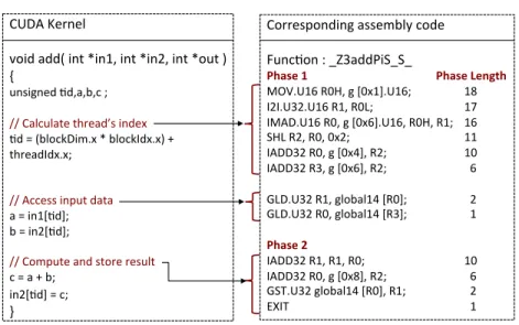
Fig. 3.2 shows an example of a simple CUDA kernel that adds two vectors. Three high

19 CUDA%Kernel% % void%add(%int%*in1,%int%*in2,%int%*out%)% {% unsigned%;d,a,b,c%;% % //%Calculate%thread’s%index%%%% ;d%=%(blockDim.x%*%blockIdx.x)%+% threadIdx.x;% % % //%Access%input%data%%%%%%%%%%%%% a%=%in1[;d];% b%=%in2[;d];% % //%Compute%and%store%result%%%% c%=%a%+%b;% in2[;d]%=%c;% }% Corresponding%assembly%code% % Func;on%:%_Z3addPiS_S_% Phase&1 % % %%%%%%%%%%%%%%Phase&Length& MOV.U16%R0H,%g%[0x1].U16; % %18% I2I.U32.U16%R1,%R0L; % % %17% IMAD.U16%R0,%g%[0x6].U16,%R0H,%R1; %16% SHL%R2,%R0,%0x2; % % % %11% IADD32%R0,%g%[0x4],%R2; % % %10% IADD32%R3,%g%[0x6],%R2; % % %%%6% % GLD.U32%R1,%global14%[R0]; % %%%2% GLD.U32%R0,%global14%[R3]; % %%%1% % Phase&2%% IADD32%R1,%R1,%R0;% % % %10% IADD32%R0,%g%[0x8],%R2; % % %%%6% GST.U32%global14%[R0],%R1; % %%%2% EXIT % % % % % %%%1%

Figure 3.2: CUDA kernel for vector addition and its corresponding assembly code showing phases and phase length.

variables that store the thread and block identifiers (threadIdx.xand blockIdx.x), and the

thread block dimension (blockDim.x). The index is then used as an offset from the base

addresses (passed as arguments to kernel call) to load data for that thread. The computation is performed and result is stored back in the third section. The right box in the figure shows the corresponding assembly code.

We define a phase as: A set of consecutive instructions such that, no instruction in the

set has any input operands that are produced by a long latency instruction from any other

instruction in the set.

Observe that this kernel has two phases (refer to Fig. 3.2). Phase 2 begins at instruction:

IADD32 R1,R1,R0. The input operandsR0 and R1 are produced by memory load instructions

(GLD), which belongs to the set of long latency instructions1. It should be noted that in

real-world application kernels, contrary to the example shown, it is common to have multiple instructions in a phase that depend on long latency instructions from the previous phase. A new phase begins only if an instruction depends on a long latency instruction from the current phase. We show a simple example here for brevity. The structure of a phase is often as follows: multiple memory loads at the beginning of a phase (initial loads), followed by computations

1

In addition to load and store, conditional and unconditional branches, and synchronization instructions are also considered as long latency instructions.

20

that depend on loads from the previous phase, and then an instruction that depends on one of the initial loads (this would begin a new phase). For the kernels we studied for this work, the number of phases in a kernel vary from 3 to 45.

3.3.2 Effect of Kernel Phases on Warp Schedulers

In the two level warp scheduler, a warp is moved from the Ready Warps queue to the larger pool of all warps, when it arrives at an instruction that depends on a long latency operation. As such instructions lie at phase boundaries, warps proceed through the kernel instructions one phase at a time. When a warp reaches the end of a phase, it is put back in the larger warp pool and a different fetch group gets a chance to execute. As the fetch group maintains its priority until it reaches the end of a phase, one of the main factors that affects the performance of the

warp schedulers is phase length (refer to Fig.3.2). Phase length is computed by summing the

instruction latencies, from the last to the first instruction of a phase. It is an approximation of the minimum number of cycles that a warp would take to reach the end of a phase. The

lengths of phases 1 and 2 in Fig. 3.2are 18 and 10 respectively.

Fig. 3.3is a depiction of the effect of phase length on performance of the warp schedulers.

For simplicity, the illustration assumes that all warps in a fetch group (FG) arrive at the end of

a phase simultaneously. Fig. 3.3(a)is an example of an application where the GTO scheduler

performs better than RR. It has a medium length phase, followed by a short phase and then phase of long length. Notice that the computation from medium length phase of FGs 2 and 3

are enough to hide the memory latency of FG 1. At this time, the RR scheduler selects FG 4 1,

while the GTO scheduler selects FG 1 2. Observe that, with RR scheduling all the FGs arrive

at the short length phase at the same time. As computation from three short length phases

is not enough to hide the memory latency, some of the latency is exposed 3. In contrast, as

the GTO scheduler selects FG 1 at 2, FG 1 arrives at the long length phase earlier 4. This

long phase is then used to hide the latency which was exposed in the case of RR scheduling. In general, for kernels that have shorter length phases in the middle of the kernel, the GTO scheduler performs better than RR.

21 FG#1# Two#Level#RR# Two#Level#GTO# FG#1# FG#2# FG#3# FG#4# FG#2# FG#3# FG#4# FG#5# 1# 2# 3# 4# FG#6# (a) Two$Level$RR$ Two$Level$GTO$ FG$1$ FG$2$ FG$3$ FG$4$ FG$1$ FG$2$ FG$3$ FG$4$ 5$ 6$ (b) )Warps)wai&ng)on))) )memory) )Warps)in)a)fetch)group))

)doing)computa&on) )Nonqoverlapped)))latency)

Figure 3.3: Impact of phase length on warp scheduling.

compared to GTO. Notice that the application has a medium phase, followed by a phase of

long length. Similar to the example of Fig. 3.3(a), computation from three FGs is enough to

hide the memory latency of FG 1, and the GTO scheduler switches back to FG 1 5. As this

phase is long enough to overlap the latency of outstanding memory requests, the load on the

memory subsystem is reduced. On the contrary, the RR scheduler selects FG 4 6. This results

in sending out more requests to memory, and thus better utilization of the memory bandwidth while executing the long length phase. We can observe that around the time when the GTO scheduler begins fetch group 4, the RR scheduler has already executed a significant portion of it. In general, for kernels that have extremely long phases in the middle of the kernel, the RR scheduler performs better than GTO.

3.3.3 Illustrative Applications

The effects of phase length on warp scheduling policies can be summarized as follows: 1. Performance of the RR policy is adversely affected in kernels that have shorter length phases,

22

due to all the warps arriving at these phases at the same time.

2. Performance of the GTO policy is adversely affected in kernels that have long length phases, as the scheduler keeps choosing warps from these phases, thereby under-utilizing the memory bandwidth.

In this section, we explore two real-world application kernels that clearly demonstrate these

effects. The top figures in each of the subplots of Fig.3.4 and Fig. 3.5plot the total number

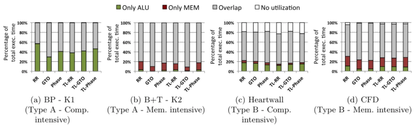
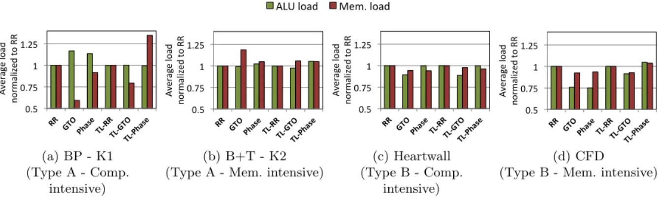
of warps in each phase at a given cycle. The bottom figure plots the total the number of ALU instructions and memory requests that are in flight.

3.3.3.1 B+Tree

B+Tree is an example of a kernel for which the GTO scheduler achieves a better performance compared to RR. It launches 48 warps on each core, as six thread blocks of eight warps each. The fetch group size is six.

Observe in Fig. 3.4(a)that, when warps from the first fetch group (FG) complete the first

phase, warps in the next FG execute. Warps completing a phase can be seen in the plot when the number of warps in a particular phase decreases. This is followed by the third FG, and so on. Thus, due to RR scheduling warps proceed through the kernel instructions one phase at a

time. As mentioned in Sect. 3.3.2, this trait of the RR scheduler becomes an issue in kernels

which have short length phases. Observe that phase 4 is extremely short (marked oval). All the warps finish this phase and arrive at the start of phase 5 at around the same time. Observe that during this time, the memory load is high and ALU load becomes almost zero. This is because all warps are waiting for the memory requests issued in phase 4. The phase problem alleviates a little after cycle 4000 due to some warps branching back to phases 1 and 3. However, only a small portion of the runtime is shown here. The application grid is of 65535 blocks and this

pattern keeps repeating throughout the kernel execution after every 6th block.

In contrast, observe in Fig.3.4(b), that after three fetch groups complete, the GTO scheduler

selects FG 1. This is observed in the figure when the number of warps in phase 1 stop decreasing and the number of warps in phase 2 start to decrease. Due to this decision, only a small set of warps arrive at the short length phase 4, at the same time. As the other warps are in the

23 P"="Phase" 10" 50" 40" 30" 20" ""0" "A c0ve " W ar ps " MEM" ALU" In str uc 0o ns " ""i n" fli gh t"

Introduction Kernel Scheduler Warp Scheduler

Thread Block Scheduler

Future Work Conclusion """"" " " """"" " " Cycles" 0""""""""1000""""2000"""""3000""""4000"""""5000""""6000"""""7000""""8000"""""9000" 0""""""""1000""""2000"""""3000""""4000"""""5000""""6000"""""7000""""8000"""""9000" Cycles" 30" 50" 40" ""0" 20" 10" 10" 30" 20" ""0" P1""" P2""" P3""" P4""" P5""" P6""" P7""" P8""" P9""" P10""" P11"""

(a) Two Level Round Robin

Cycles' 'A c)ve ' W ar ps ' MEM' ALU' In str uc )o ns ' ''in' fli gh t'

Introduction Kernel Scheduler

Warp Scheduler Future Work

Conclusion

Cycles' _{ALU' MEM'}

Cycles' 0''''''''1000''''2000'''''3000''''4000'''''5000''''6000'''''7000''''8000'''''9000' Cycles' 0''''''''1000''''2000'''''3000''''4000'''''5000''''6000'''''7000''''8000'''''9000' ''''' ' ' 30' 50' 40' ''0' 20' 10' ''''' ' '10' 30' 20' ''0' P'='Phase' P1''' P2''' P3''' P4''' P5''' P6''' P7''' P8''' P9''' P10''' P11'''

(b) Two Level GTO

Figure 3.4: B+Tree Phase Graphs

longer length phases, the scheduler can switch to them to hide the memory latency. Observe

in the lower plot of Fig. 3.4(b), the amount of time when the ALU and memory load becomes

zero has reduced as compared to the RR scheduler. Moreover, observe in the area plot that the distribution of warps across different phases (marked oval) is much better in GTO as compared to RR.

3.3.3.2 Computational Fluid Dynamics (CFD)

CFD is an example of a kernel for which RR scheduling achieves better performance as compared to GTO. It launches 18 warps on each core, as three thread blocks of 6 warps each.

Observe in Fig. 3.5(b) that the first fetch group (FG) of 6 warps starts executing ahead and

reaches phase 2. Notice that the GTO scheduler selects FG 1 again (first marked oval). This is because, as phase 1 is a long length phase, the memory requests sent near its beginning are completed by the time warps reach phase 2. As the next two phases are long as well, the warps in FG 1 become pending only when they reach phase 4. At this time fetch group 2 gets to

24 !A c$ve ! W ar ps ! MEM! ALU! In str uc $o ns ! !!i n! fli gh t!

Introduction Kernel Scheduler Warp Scheduler Future Work

Conclusion !!!!! ! ! Cycles! Cycles! 20! !!0! 10! P!=!Phase! P1!!! !!!!! ! ! 40! 20! !!0! P2!!! P3!!! P4!!! P5!!! P6!!! P7!!! P8!!! P9!!! 10000! 20000! 30000! 40000! 45000! 0! 10000! 20000! 30000! 40000! 45000! 0!

(a) Two Level Round Robin

!A c$ve ! W ar ps ! MEM! ALU! In str uc $o ns ! !!i n! fli gh t!

Introduction Kernel Scheduler Warp Scheduler Future Work

Conclusion !!!!! ! ! Cycles! Cycles! 20! !!0! 10! P!=!Phase! P1!!! !!!!! ! ! 40! 20! !!0! P2!!! P3!!! P4!!! P5!!! P6!!! P7!!! P8!!! P9!!! 10000! 20000! 30000! 40000! 45000! 0! 10000! 20000! 30000! 40000! 45000! 0!

(b) Two Level GTO

Figure 3.5: CFD Phase Graphs

execute. Observe that when warps from FG 2 reach phase 2 and become pending, FG 1 gets selected again and executes until it reaches phase 6 (second marked oval).

In this manner, due to phases of long length, a group of warps keeps getting the priority. Consequently, other warps do not get a chance to execute and issue their memory requests.

Observe in the lower plot of Fig. 3.5(b) that the memory load becomes zero in the duration

when warps from FG 1 are in the long compute phases. In comparison, the RR scheduler switches priority to the next fetch group at phase boundaries. Due to this, warps that were in the shorter length phases are able to execute and send the memory requests. We can observe in Fig.3.5(a) that the warp distribution across different phases is much better. Also, notice that the memory load is more regular and has lesser fluctuations as compared to GTO. The average memory load for this kernel with the two level RR scheduler was 4% higher as compared to the two level GTO.

25

3.4 Phase Aware Warp Scheduling

In this section, we first propose a dynamic scheduling policy based on phase length that can mitigate the negative effects of phases outlined in the previous section. We then provide details of the compiler frontend that adds the required phase information in program instructions and hardware implementation of the warp scheduler that uses this information at runtime.

3.4.1 Scheduling Policy

In the previous section, we showed that performance of the RR scheduler is affected if the kernel has phases of short length and all the warps arrive at such phases simultaneously. On the other hand, performance of the GTO scheduler is adversely affected when the kernel has long phases and the scheduler keeps selecting the set of warps that are in the long phase.

Our policy is based the following simple observation: Adverse effects of the RR and GTO

scheduling policies can be mitigated by always choosing the warp that is at the shortest next

phase.

Consider a kernel with two phases Pi and Pj, such thatPj is shorter thanPi.

Case (1): The RR policy chooses a warp in phase Pi. This implies that warps in Pj were

selected before this.

(a): Pi is beforePj in program order. This is the more common case given that warps in Pj

were selected earlier. Selecting warps in phasePi would get all warps to the shorter phasePj,

leading to a possibility of non-overlapped memory latency. Hence, it would be ideal to first

select warps in Pj.

(b): Pi is after Pj in program order. This would happen if warps (currently in Pj) executed

before this and branched back to an earlier phase. Selecting warps in phase Pj would get all

warps to the longer phase Pi. Note that in this case, selecting warps from Pi would harm

performance only if they branch back to phase Pj. Nonetheless, selecting warps in Pj would

not negatively impact performance.

Case (2): The GTO policy chooses a warp in phasePi. This implies that warps in Pi were

26 Ac#ve&Warps&Queue& Ready&Warps& If#space,#move## head#of#queue## to#ready#warp# Warp&selec#on&logic& To#execu7on#units# Pending&Warp&Queue& Move#if#long#latency### instruc7on#completes# Priority&Assignment&Logic&

Figure 3.6: Block diagram of our two level warp scheduler.

(a): Pi is after Pj in program order. This is the common case as GTO gives priority to older

warps, causing them to be ahead in the program. If phase Pi is extremely long, choosing a

warp from phasePi might under-utilize the memory bandwidth. Hence, it would be better to

first execute warps inPj and then overlap the memory latency using warps in phase Pi.

(b): Pi is before Pj in program order. This would happen if warps with the lower index have

branched back to Pi. Again, selecting warps in phase Pj would issue memory requests which

can then be overlapped by warps fromPi. Note that in this case, selecting warps fromPi would

have the same effect, if warps inPj also branch back toPi. Nonetheless, selecting warps which

are in phasePj would not negatively impact performance.

3.4.2 Implementation

3.4.2.1 Front-end

The phase length information is computed at compile time and included in the kernel

instructions. As the CUDA ISA is not open-source, we use PTX-Plus [10]. PTX is an

intermediate assembly language generated during the compilation of CUDA kernels. PTX-Plus is a modified version of PTX which closely matches the ISA that executes on the hardware. We

27

chose to work with PTX-Plus because we observed that PTX is generated before the compiler has performed instruction scheduling. Due to this, the memory load and store instructions are scheduled very close to their dependent instructions, resulting in the instruction sequence being fragmented into several phases.

A long-op register is defined as a register that is a destination operand of a long latency instruction. To create phases, a set of long-op registers (empty at initialization) is maintained. The PTX-Plus assembly code is parsed at compile time from top to bottom and long-op registers are added to the set one instruction at a time. The first instruction that consumes any register currently in the set marks the start of a new phase. At the start of each phase, the set is cleared. This assumes that long latency instructions issued close to each other would complete around the same time, and avoids creating several short phases. In addition, each basic block starts a new phase.

Once the phases are created, the code is traversed backwards to calculate phase lengths. Within each phase, instruction latencies are accumulated from the last to the first instruction

as mentioned in Sect. 3.3.1. This simultaneously calculates two pieces of information. Each

instruction is assigned a phase distance, which approximates the number of cycles a warp executing this instruction would take to reach the end of the phase. Additionally, each phase is assigned a phase length, which approximates the number of cycles a warp takes to execute the phase.

3.4.2.2 Hardware Implementation

The schedulers were implemented in GPGPU-Sim v3.2 [10], a cycle-accurate GPU architecture simulator. The phase distance mentioned in the previous subsection is used by the phase-aware single level scheduler, while the phase length is used by the phase-aware two level scheduler.

Single Level Schedulers: As mentioned in Sect. 3.2, single level schedulers maintain a queue of all warps that are active on a core. All the warps in the active queue are checked every cycle and the one with the highest priority is chosen. The priority assigning policy is the key difference between the different schedulers. The RR scheduler rotates the priority after each selection, while the GTO scheduler always assigns the highest priority to the oldest warp. The

28

phase aware scheduler compares the phase distance of the current instruction for each warp. Warp at an instruction with the lowest distance from the next phase is chosen. For warps that are at the same distance, the oldest warp is chosen first. This requires the distance information to be added for each instruction. In real GPU implementations, this can be achieved via opcode extensions. Our experiments showed that a phase distance of 512 covers more than 98% of all

kernels2. Considering instruction size of 8 bytes and L1 cache line size of 128 bytes, adding

phase distance would increase the static instruction size by 12.5%.

Two Level Schedulers: In the baseline two level scheduler (refer to Fig. 3.1), when a warp in the ready queue arrives at a long latency operation, it is put in the active queue and replaced by the warp from the head of the queue. This implementation works well if priority of the warps in the active queue is rotated in a round robin order. However, notice that this is an issue for any scheme that requires warps to be prioritized. If a single queue is used to store the active warps, as well as the warps waiting on long latency operations, all the warps would need to be checked when replacing a warp from the ready queue. To solve this, we use an additional pending queue to store warps that are waiting on long latency instructions.

Fig. 3.6 shows a block diagram of our implementation of the two level scheduler. A warp

waiting on a long latency instruction is first moved to the pending queue. When all the

long latency instructions complete, it is moved to the tail of the active queue. The priority assignment logic is triggered at this point and warps in the active queue are sorted. This design effectively allows implementation of different scheduling policies by modifying the policy of the priority assignment logic. The RR scheduler does not sort the warps, while the GTO scheduler sorts the warps in launch order. The phase-aware scheduler uses the phase distance of the next phase to sort the warps. Consequently, contrary to the single level scheduler, length information is required only once for an entire phase. Our experiments show that adding phase length increases the static instruction size by less than 1%. After sorting, warp at the head of the active queue is moved to the ready queue.

29

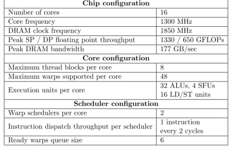
Table 3.1: GPGPU-Sim configuration used for evaluating phase aware warp scheduler Chip configuration

Number of cores 16

Core frequency 1300 MHz

DRAM clock frequency 1850 MHz

Peak SP / DP floating point throughput 1330 / 650 GFLOPs

Peak DRAM bandwidth 177 GB/sec

Core configuration

Maximum thread blocks per core 8

Maximum warps supported per core 48

Execution units per core 32 ALUs, 4 SFUs

16 LD/ST units

Scheduler configuration

Warp schedulers per core 2

Instruction dispatch throughput per scheduler 1 instruction every 2 cycles

Ready warps queue size 6

3.5 Experimental Results

3.5.1 Methodology

We configured the simulator [10] to match the architecture of NVIDIA Tesla M2090 GPU

[53] (refer to Table 3.1). To perform our evaluations we chose kernels from the CUDA SDK

[51] and the Rodinia benchmark suites [14]. The SDK has 49 applications, while Rodinia has 19; with each application having multiple kernels. We pruned our workload list by omitting the applications provided in the SDK for hardware profiling and demonstrating interoperability with graphics APIs. We also omitted kernels that did not have a grid size large enough to fill all the cores, and the size could not be increased without significantly changing the application code. Our final workload list had 13 kernels from 11 applications of the SDK and 17 kernels

from 12 applications of Rodinia (refer to Table3.2and Table3.3). For brevity, we discuss results

of kernels for which either the RR or the GTO scheduling policy showed a better performance. For the remaining kernels, the GTO, RR and phase-aware scheduling policies had comparable performance (within 1% of each other).

30

Table 3.2: Workloads from the Rodinia benchmark suite [14] used for evaluating phase aware warp scheduler

Name Back B+Tree Heart K-means LU Decom- Speckle Reducing Comp.Fluid

Propagation Search Wall Clustering position Anisotropic Diff. Dynamics

Abbreviation BP - K1 BP - K2 B+T - K1 B+T - K2 Heart KM LUD SRAD CFD

Total Thread Blocks 65535 65535 65535 65355 56 841 16129 16384 1817

Threads / Block 256 256 256 256 256 256 256 256 192

Thread Blocks / Core 6 5 5 6 4 6 6 6 3

Total Phases 5 5 16 11 45 2 3 4 9

Longest Phase 206 99 40 32 212 48 150 218 985

Shortest Phase 26 14 5 3 41 14 7 31 86

Table 3.3: Workloads from the CUDA SDK [51]

Name Discrete Wavelet DXT Fast Walsh Histogram Monte Carlo Transform Compression Transform Option Pricing

Abbreviation DWT DXTC FWT HIST MCO

Total Thread Blocks 4096 4096 4096 256 2048

Threads / Block 512 256 512 192 256

Thread Blocks / Core 3 4 3 6 5

Total Phases 2 3 2 2 2

Longest Phase 144 1159 174 44 284

Shortest Phase 44 24 45 24 38

3.5.2 Impact on Performance

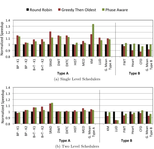
Fig. 3.7 plots the speedup of the Greedy Then Oldest (GTO) and phase-aware schedulers

normalized to the Round Robin (RR) scheduler. The single level schedulers have an advantage of selecting from all the warps on the core. Hence, we compare the performance of the single level and two level schedulers separately. We have grouped the kernels into two types. For

kernels grouped under Type A, the GTO scheduler achieves a better performance compared

to RR, while for kernels grouped underType B, the RR scheduler performs better than GTO.

3.5.2.1 Type A Kernels

Kernels for which the GTO policy performs better (grouped under type A), have phases of

extremely short length. As mentioned in subsection3.3.3.1, our simulations showed that when

the RR policy is used, warps get accumulated in these short phases at around the same time, causing the core to become idle.

Eight kernels always perform better with the GTO policy (refer to Fig. 3.7(a)). The

BP-K2, DWT, HIST and MCO kernels have their shortest phase at the beginning of the kernel. The SRAD kernel has two short phases in the middle of the kernel code, while the B+Tree kernels have phases of length shorter than 20 cycles intermixed throughout the code. Notice

31 BP#$#K1# BP#$#K2# _B+T#$# K1 # B+T #$# K2 # SRA D #$# K5 # SRA D #$# K6 # DW T#$#K 1# D XT C# FW T#$#K 5## Hi st# K5 # He ar t# KM# $#K 2# LU D#$#K 3# CFD#$#K 5# Hi st# $#K 5# MC O #$# K2 # G .#Me an #

Round#Robin# Greedy#Then#Oldest# Phase#Aware#

0.8$ 0.9$ 1$ 1.1$ 1.2$ 1.3$ 1.4$ BP$,$K1$ BP$,$K2$ _B+T$,$ K1 $ B+T $,$ K2 $ SRA D $ DW T$ D XT C$ HIS T$ MC O $ KM$ _LUD$ G .$Me an $$$ $$$ $$$ $$$ $ Ty pe $A $ FW T$ He ar t$ CFD$ G .$Me an $$$ $$$ $$$ $$$ $$$ $$$ $$$ $$$ $$$ $ Ty pe $B$ N or m al ize d$ Sp ee du p$ Type%A% Type%B%

(a) Single Level Schedulers

0.8$ 0.9$ 1$ 1.1$ 1.2$ 1.3$ 1.4$ BP$,$K1$ BP$,$K2$ _B+T$,$ K1 $ B+T $,$ K2 $ SRA D $ DW T$ D XT C$ HIS T$ MC O $ G .$Me an $$$ $$$ $$$ $$ Ty pe $A $ KM$ _LUD$ _FWT$ He ar t$ CFD$ G .$Me an $$$ $$$ $$$ $$$ $$ Ty pe $B$ N or m al ize d$ Sp ee du p$ Type%A% Type%B%

(b) Two Level Schedulers

Figure 3.7: Performance comparison. Type A - GTO performs better than RR. Type B

-RR performs better than GTO.

in Fig. 3.7 that the BP-K1, LUD and KM kernels have a better performance with the GTO

policy for single level implementation and with the RR policy for two level implementation. This happens due to a phenomenon we refer to as intra-block tail effect, which we will explain

in detail in subsection 3.5.5.

For the type A kernels, the single level GTO has a speedup of 10% over single level RR on average. The performance of the phase-aware scheduler is close to that of GTO for all these kernels and it achieves a speedup of 9% on average over RR. A similar performance trend was observed for the two level schedulers. However, as warps progress through the kernel in fetch groups, all the warps do not arrive at the short phases simultaneously. This reduces

the negative effect on performance of the RR scheduler. Notice in Fig. 3.7(b) that for the

phase-32

aware. Consequently, the speedup of GTO over RR is lesser with an average of 4%. Again, the performance of the phase-aware scheduler is close to that of GTO and it achieves a speedup of 3% on average over RR.

3.5.2