WIND SPEED FORECASTING FOR POWER SYSTEM OPERATION
A Dissertation by XINXIN ZHU
Submitted to the Office of Graduate and Professional Studies of Texas A&M University
in partial fulfillment of the requirements for the degree of DOCTOR OF PHILOSOPHY
Chair of Committee, Huiyan Sang Co-Chair of Committee, Marc G. Genton Committee Members, Raymond J. Carroll
Le Xie
Head of Department, Simon J. Sheather
August 2013
Major Subject: Statistics
ABSTRACT
In order to support large-scale integration of wind power into current electric energy system, accurate wind speed forecasting is essential, because the high varia-tion and limited predictability of wind pose profound challenges to the power system operation in terms of the efficiency of the system. The goal of this dissertation is to develop advanced statistical wind speed predictive models to reduce the uncer-tainties in wind, especially the short-term future wind speed. Moreover, a criterion is proposed to evaluate the performance of models. Cost reduction in power system operation, as proposed, is more realistic than prevalent criteria, such as, root mean square error (RMSE) and absolute mean error (MAE).
Two advanced space-time statistical models are introduced for short-term wind speed forecasting. One is a modified regime-switching, space-time wind speed fore-casting model, which allows the forecast regimes to vary according to the dominant wind direction and seasons. Thus, it avoids a subjective choice of regimes. The other one is a novel model that incorporates a new variable, geostrophic wind, which has strong influence on the surface wind, into one of the advanced space-time statistical forecasting models. This model is motivated by the lack of improvement in forecast accuracy when using air pressure and temperature directly. Using geostrophic wind in the model is not only critical, it also has a meaningful geophysical interpretation. The importance of model evaluation is emphasized in the dissertation as well. Rather than using RMSE or MAE, the performance of both wind forecasting models mentioned above are assessed by economic benefits with real wind farm data from Pacific Northwest of the U.S and West Texas. Wind forecasts are incorporated into power system economic dispatch models, and the power system operation cost is
used as a loss measure for the performance of the forecasting models. From another perspective, the new criterion leads to cost-effective scheduling of system-wide wind generation with potential economic benefits arising from the system-wide generation of cost savings and ancillary services cost savings.
As an illustration, the integrated forecasts and economic dispatch framework are applied to the Electric Reliability Council of Texas (ERCOT) equivalent 24-bus system. Compared with persistence and autoregressive models, the first model suggests that cost savings from integration of wind power could be on the scale of tens of millions of dollars. For the second model, numerical simulations suggest that the overall generation cost can be reduced by up to 6.6% using look-ahead dispatch coupled with spatio-temporal wind forecast as compared with dispatch with persistent wind forecast model.
ACKNOWLEDGEMENTS
First, I would like to express the deepest appreciation to my advisor Dr. Marc G. Genton, an outstanding statistician in multiple fields, particularly, in spatial-temporal statistics and skew-slliptical sistributions area. As an advisor, he is in-spirational, supportive, helpful and patient throughout my four years’ PhD study. Without his guidance and persistent help this dissertation would not have been pos-sible. Moreover, with his attitude to research work, he sets a great model for me to follow in my future life.
I also very much appreciate Dr. Huiyan Sang, who agreed to become my advisor for the last year. Her warmth and kindness have been great support for me at the end of my PhD study. As a young statistician of my age, Dr. Sang has already attained her prominent achievements in extreme value study, which inspires me to work harder.
I would like to thank my committee members, Dr. Raymond J. Carroll and Dr. Le Xie. I thank Dr. Xie and his student, Yingzhong Gu, for their great efforts, help, and comments on the join works, for giving me opportunities to share and discuss my researches in their group. Without them this dissertation would not have been finished. I also thank Dr. Kenneth Bowman’s great guidance and technical assistance in one important part of my dissertation. I am also very grateful to Dr. Michael Longnecker, the associate Department Head, for his constant help on problems I met through the process of completing my PhD program. In addition, I very much thank my mentor, Dr. Suojin Wang, for his valuable advises on my PhD study and personal life, which I will cherish in my future life.
and my friends for their unconditional and endless support. They have been always with me through ups and downs during my PhD study. Thank you.
TABLE OF CONTENTS Page ABSTRACT . . . ii ACKNOWLEDGEMENTS . . . iv TABLE OF CONTENTS . . . vi LIST OF FIGURES . . . ix
LIST OF TABLES . . . xii
1. INTRODUCTION . . . 1
2. LITERATURE REVIEW . . . 7
2.1 Introduction . . . 7
2.1.1 Wind Energy . . . 7
2.1.2 Integrating Wind Energy into the Power System . . . 10
2.1.3 Outline . . . 12
2.2 Wind Speed Forecasting . . . 13
2.2.1 Wind Speed and Power Forecasting . . . 14
2.2.2 Point Forecasting Versus Probabilistic Forecasting . . . 15
2.2.3 Space-Time Wind Correlations . . . 18
2.3 Time Series Models for Forecasting . . . 19
2.3.1 Basic Concepts . . . 19
2.3.2 Reference Model . . . 20
2.3.3 Autoregressive Models . . . 20
2.3.4 Kalman Filter . . . 22
2.4 Space-Time Statistical Models for Forecasting . . . 24
2.4.1 Motivation . . . 24
2.4.2 Regime-Switching Space-Time Diurnal Model . . . 25
2.4.3 Trigonometric Direction Diurnal Model . . . 28
2.4.4 Other Models . . . 29
2.5 Evaluation of Forecasts . . . 30
2.5.1 Loss Functions and Forecasts . . . 30
2.5.2 Realistic Loss Functions for Wind . . . 32
2.5.3 Comparison of Forecast Accuracy . . . 35
2.5.4 Uncertainty of Forecasts . . . 36
2.6.2 Offshore Wind Speed Forecasting . . . 38
2.6.3 Final Remarks . . . 39
3. ROTATING SPACE-TIME REGIME-SWITCHING WIND SPEED FORE-CASTING FOR IMPROVED POWER SYSTEM DISPATCH . . . 42
3.1 Introduction . . . 42
3.1.1 Wind Energy . . . 42
3.1.2 Wind Speed Forecasting . . . 43
3.2 The Rotating RSTD Model . . . 46
3.2.1 RRSTD Model Description . . . 46
3.2.2 Reference Models . . . 49
3.3 Numerical Experiments . . . 50
3.3.1 Wind Data . . . 50
3.3.2 Exploratory Data Analysis . . . 51
3.3.3 Training Data Results . . . 52
3.3.4 Testing Data Results . . . 54
3.4 Integrating Wind Power into a Power System . . . 56
3.4.1 Power System Specification in the BPA Region . . . 56
3.4.2 Power System Dispatch with Space-Time Wind Forecasts . . . 58
3.4.3 A Realistic Illustrative Example . . . 62
3.4.4 Analysis of Economic Dispatch Results . . . 65
3.5 Conclusion . . . 70
4. INCORPORATING GEOSTROPHIC WIND INFORMATION FOR IM-PROVED SPACE-TIME SHORT-TERM WIND SPEED FORECASTING 72 4.1 Introduction . . . 72
4.2 Estimating the Wind in the Free Troposphere . . . 75
4.3 The Trigonometric Direction Diurnal Model with Geostrophic Wind . 80 4.3.1 The TDD Model . . . 80
4.3.2 The TDDGW Model . . . 82
4.3.3 Reference Models . . . 84
4.4 West Texas Data . . . 84
4.4.1 Data Description . . . 84
4.4.2 Data Exploration . . . 86
4.4.3 Geostrophic Wind and Surface Wind . . . 88
4.5 Numerical Results . . . 92
4.5.1 Training Results . . . 92
4.5.2 Evaluation of Forecasts . . . 94
4.6 Final Remarks . . . 97
5. SHORT-TERM SPATIO-TEMPORAL WIND POWER FORECAST IN LOOK-AHEAD POWER SYSTEM DISPATCH . . . 99
5.1 Introduction . . . 99
5.2.1 Wind Data Source in West Texas . . . 102
5.2.2 Space-time Statistical Forecasting Models . . . 103
5.3 Forecasting Results and Comparison . . . 105
5.4 Power System Dispatch Model . . . 107
5.4.1 The Two-layer Dispatch Model . . . 107
5.4.2 Procurement of Operating Reserves . . . 112
5.5 Numerical Experiment . . . 114
5.5.1 Simulation Platform Setup . . . 114
5.5.2 Results and Analysis . . . 117
5.6 Conclusions . . . 122
6. SUMMARY . . . 124
LIST OF FIGURES
FIGURE Page
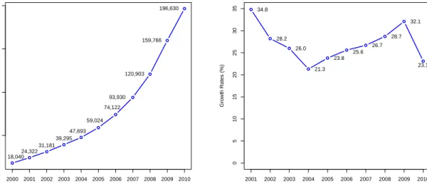
2.1 Left panel: world total installed wind power capacity from year 2000 to 2010. Right panel: world market growth rate of newly installed wind power capacity from the installed capacity of the previous year during 2000 to 2010. . . 8 2.2 Country shares of total installed wind power capacity (in MW and
percentage) by the end of 2010. . . 9 2.3 Three power curves with different capacity ranges from low to high
from three manufacturers: 0.3 MW from Nordex, 1.5 MW from GE, and 2.5 MW from Bonus. . . 14 2.4 Nonparametric density estimation of 2002 hourly wind speed data at
Vansycle, Oregon, U.S. The vertical lines represent the sample mean (solid) of 6.6 m/s and the sample median (dashed) of 5.4 m/s. The sample skewness is 0.8. . . 16 2.5 Map of the three locations: Vansycle, Kennewick and Goodnoe Hills
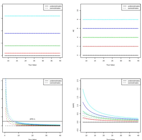
on the border between Washington and Oregon in the U.S.. . . 26 2.6 Squared error (SE), absolute error (AE), absolute percentage error
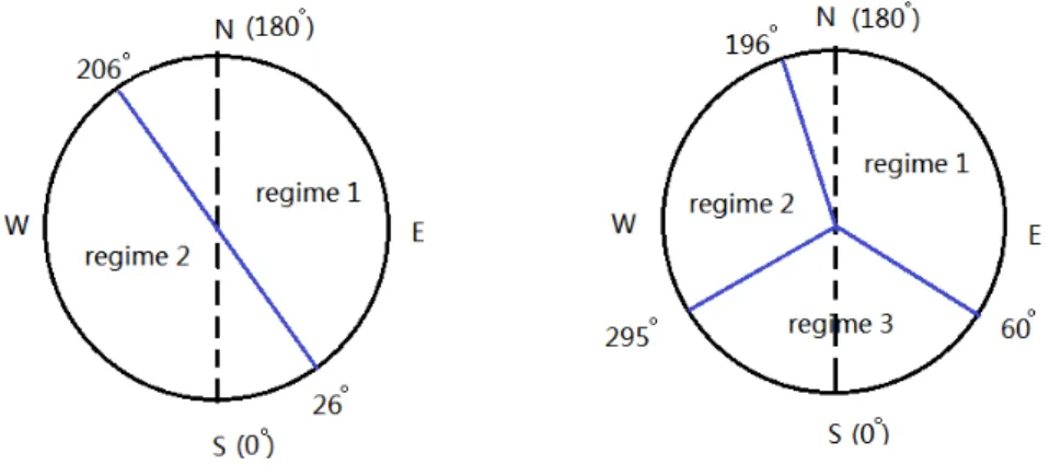
(APE) and symmetric absolute percentage error (SAPE) for forecasts of true valuesy= 8,8.5,9,9.5, . . . ,40 with prediction errors 0 (black), 2 (red), 4 (green), 6 (blue), 8 (cyan) for each. Overestimates for extra true values 0,0.5,1, . . . ,7.5 with prediction errors 0,2,4,6,8 are generated for APE. . . 34 3.1 Regime dividing plots forθ∗m(t+k)={26◦,206◦}Aug(left) andθ∗m(t+k)=
{60◦,196◦,295◦}Aug (right). The dashed line connects the south (0◦) and the north (180◦), with the westerly wind to the left and the east-erly wind to the right. Separate models of µrs,t+kare built for each regime. . . 48
3.3 Plots of 1-hour-ahead prediction MAE results based on the two-regime RRSTD model with the dividing angle, θ, from 0◦ to 180◦ for each month at Vansycle in 2002. The blue dashed line indicates the position of the best two-regime dividing angle, orθ∗, that has the smallest MAE value. . . 52 3.2 Wind roses of data from August to November 2002 at Vansycle (left
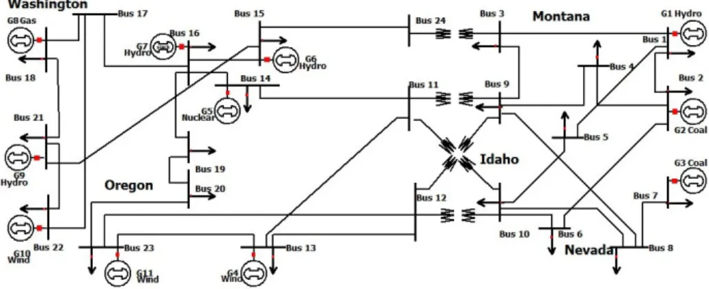
column), Kennewick (middle column) and Goodnoe Hills (right col-umn). . . 53 3.4 BPA’s scheduling procedure [Makarov et al., 2008]. . . 57 3.5 A system network diagram with BPA’s operation areas. This network
has 24 electrical nodes and 11 power generators including hydro, coal, nuclear, natural gas and wind power. The installed generation capac-ity in the simulation system is configured according to the resources listed in Table 3.3. . . 63 3.6 The wind generation potential of Vansycle, Kennewick and Goodnoe
Hills on 15 August 2003. The horizontal axis indicates different time steps with 10 minutes per interval, and the vertical axis indicates the wind production potential or available wind generation in MW. . . . 64 3.7 Histograms of relative cost savings in percentage based on wind power
forecasts from the AR and RRSTD models, compared with the costs based on forecasts from PSS. . . 68 3.8 Actual wind generation at Kennewick (top panel), total system
re-serve service requirement (middle panel), and total system regulation service requirement (bottom panel) on 15 August 2003, for different forecasting approaches including OB, PSS, AR, and RRSTD models. 69 4.1 The pressure gradient force, Coriolis force, and friction force influence
the movement of air parcels near the ground. Geostrophic balance (left) and higher-order balance including friction (right). . . 77 4.2 The distribution of Mesonet Towers (stars) in West Texas and Eastern
New Mexico. . . 85 4.3 Wind roses of wind speeds in 2008-2009 at PICT, JAYT, SPUR, and
ROAR. . . 87 4.4 Density plots of wind speeds at PICT, JAYT, SPUR, and ROAR in
4.5 Histograms and scatter plots of approximation of geostrophic wind
components,ug and vg. . . 89
4.6 Geostrophic wind (GW) vs. surface wind (SW) (top) and density plots of the geostrophic wind and surface wind (bottom). . . 90
4.7 Scatter plots of wind speed vs. temperature (left), pressure (middle), and geostrophic wind speed (right). . . 91
4.8 Daily pattern of wind speed (lower part in each plot) and geostrophic wind speed (upper part in each plot) in different seasons of 2008 and 2009. . . 92
5.1 Map of the four locations in West Texas . . . 103
5.2 Two-layer dispatch model . . . 109
5.3 The IEEE RTS-24 system (modified) . . . 115
5.4 Distribution of forecast errors under different forecast models . . . 118
5.5 Total operating cost using different forecast models (Case A) . . . 119
5.6 Operating cost reduction using different forecast models (Case A) . . 120
LIST OF TABLES
TABLE Page
3.1 MAE values of forecasts in the 2003 testing data set based on the two-regime RRSTD models for 1-hour-ahead forecasting at Vansycle, Kennewick and Goodnoe Hills, compared with the PSS and AR mod-els. The smallest MAE values are in bold. . . 55 3.2 Notation for the power system dispatch model. . . 60 3.3 BPA’s integrated resources [BPA, 2010]. . . 63 3.4 Each generator’s configuration including capacity, marginal cost, and
ramping rates. . . 64 3.5 Economic performance (in $) of wind forecast methods for several days
in 2003. The smallest cost is in bold. . . 66 3.6 System operating results (in $) on 15 August 2003. The smallest cost
is in bold. . . 66 4.1 Information on 12 sites in West Texas. The four stations in boldface
type provide the data used in the forecast experiments. . . 86 4.2 Correlation coefficients between yP,t+2 and the current and up to
5-step lag surface wind speed (y), direction (θ), geostrophic wind speed (gw) and geostrophic wind direction (gθ) at four stations (P, J, S, and R). . . 93 4.3 MAE values of 2-hour-ahead forecasts from TDDGW with different
diurnal component fitting methods at PICT, 2010. The smallest MAE value of each column is in boldface. . . 94 4.4 MAE values of 2-hour-ahead forecasts from various forecasting models
at PICT, JAYT, SPUR, and ROAR, 2010. The smallest MAE value of each column is in boldface. . . 95 4.5 Relative (to PSS) MAE values of 2-hour-ahead forecasts from various
forecasting models at PICT, JAYT, SPUR, and ROAR, 2010 (%). The largest value of each column is in boldface. . . 96
5.1 Site information . . . 102
5.2 MAE values of the 10-minute-ahead, 20-minute-ahead and up to 1-hour-ahead forecasts on 11 days’ in 2010 from the PSS, AR, TDD and TDDGW models at the four locations (smallest in bold) . . . 106
5.3 Notations . . . 108
5.4 Generator parameters . . . 116
5.5 Sample days in simulation study . . . 116
1. INTRODUCTION
Driven by environmental concerns, energy independence, and limitation of fossil fuel resource, wind has become one of the most promising alternative energy re-sources. The main motivation for many countries to use wind energy is to reduce the emission of greenhouse gases, which is threatening the Earth by global warming. 72% of the totally emitted greenhouse gas is carbon dioxide (CO2), which is due to the burning of fossil fuels, e.g. coal, oil, natural gas; they have been the major energy resources for human activities for hundreds of years. In addition, the uneven distri-bution of such resources is the root that causes a lot of conflicts between countries and regions. The development of wind energy as an alternative is not only needed but necessary.
Wind energy is green, renewable, and rich in resource, and with advanced tech-nologies, it becomes more and more cost-effective. Unlike in old times when wind energy is used to grind grain or pump water, today’s techniques allow us to convert wind energy into power or electricity. Due to the uneven heating of the sun, the mo-tion of air or wind rotates the wind turbines, converting the kinetic energy in wind into mechanical energy. Then, electricity is converted from mechanical energy by the rotating magnetic coil in the gearbox, and finally transmitted to community. In the procedure, wind is the only input, which is very rich in nature, and the electric-ity is generated without any emission of greenhouse gases. Even the wind turbines and towers are recyclable without causing any pollution. Moreover, the innovation in wind turbine design enables us to capture more wind energy than before, e.g. smoother and stronger wind in higher altitude and off-shore. With current sophis-ticated techniques, the monetary cost per unit of energy produced is similar to the
cost for new coal and natural gas installations.
The wind industry has been growing by leaps and bounds in the last decades. By the end of 2012, 83 countries in the world are using wind power on a commercial basis. The world total installed capacity has reached 282,587 megawatt (MW), compared with 18,084 MW in 2000. Among all countries, China, the U.S, Germany, and Spain have the most rapid development of wind energy. In Chapter 2, more facts about wind energy are introduced.
However, “increased wind power cannot simply be added to the existing grid without transforming the grid in ways that introduce both significant costs and op-erational inefficiencies”, as Haugen and Musser (2012) said. Subject to the high intermittency in wind power, the stability and reliability of the power system are undermined, with costly non-wind backup power, reserve and ancillary services. Un-like other conventional power sources, wind cannot be turned on and off to meet the changes in demand, and the wind power must be used when the wind is actually blowing, due to the lack of feasible energy storage options. In a power system with a high share of wind power, the operation of standby fast power plants is costly, if the wind is not generating electricity as expected.
Therefore, to keep the cost of wind power as low as possible, it is critical to improve the accuracy of wind forecasting, especially, to reduce the uncertainties in the near-term future wind. Compared with long-term (days or longer ahead) wind forecasts, which are hardly accurate, short-term (hours-ahead) ones have higher qual-ity, and are more closely related with power system operation. Through day-ahead, hours-ahead, and even minutes-ahead electricity market, power system dispatch de-cides the amount of supply of each power plant at a minimum cost to match the demand. The more accurate hours-ahead wind forecasting is, the more efficiency the power system operation has. More importantly, it allows enough time to start
slower but less expensive power plants to make up possible gaps between demand and supply. Thus, accurate short-term wind forecasting is necessary to reduces the cost for reserve and stabilize the power system.
To provide feasible solutions, researchers have devoted time to short-term wind speed forecasting problems. Physical models, statistical models, and the combina-tion of the two areas have been applied to wind prediccombina-tion. For short-term wind forecasting, statistical models are considered to be the best. And among all statis-tical models, such as neural networks, fuzzy logic, local regression and time series methods, space-time models are the best because of high forecasting accuracy and friendly model interpretations. The advantages in space-time statistical models are attributed to their abilities to capture the spatial correlation in wind, besides that in time, by incorporating wind information of neighbors. Moreover, the prediction is in the form of probability distribution, instead of point forecasts, providing more information to reduce the uncertainties of wind. A comprehensive review for short-term wind forecasting in power system operation is in Chapter 2, including literature reviews, essential aspects in model development and future work.
The objective of this dissertation includes developing space-time statistical short-term probabilistic wind speed forecasting models, as well as proposing a new criterion to evaluate the model performance. The main contributions of this dissertation are as follow.
• A space-time statistical model is proposed aiming to generalize the regime-switching space-time diurnal (RSTD) model (Gneiting et al. 2006). In the RSTD model, two forecast regimes were predefined according to local prevail-ing wind direction, and separate forecastprevail-ing models were developed based on spatial and temporal information. It outperformed persistence and
autore-gressive forecasts in terms of RMSE, in 2-hour-ahead wind speed prediction problems at Vansycle, Oregon.
However, the definition of forecasting regimes in the RSTD model is subjective and not unique. For other situations, under which the winds follow more com-plicated patterns, the number and position of the forecast regimes are difficult to determine. To eliminate these constraints, the proposed model generalizes the RSTD model by allowing the forecast regimes to vary with the dominant wind direction in each season instead of fixing the forecast regimes based on prior geographic information. By rotating the dividing angles of the regimes with respect to the minimum MAE for each season, the best position of the forecast regimes is detected. The new model is named RRSTD short for rotat-ing RSTD.
• Another proposed space-time statistical model is called TDDGW model. It is constructed to improve the trigonometric direction diurnal (TDD) model, which was developed by Hering and Genton (2010) to generalize the RSTD model by treating wind direction as a circular variable. It obtains equivalent or better forecasting results than those from the RSTD model without requir-ing prior wind information. However, the forecastrequir-ing error is not reduced by including additional weather information directly into the model, such as air pressure and temperature, which are considered to be closely related to wind. Based on atmospheric dynamics, a new variable, the geostrophic wind, is incor-porated into the TDD model. Geostrophic wind is the airflow under geostrophic balance, a balance between the horizontal pressure gradient force and the Cori-olis force, which arises from the rotation of the Earth. It is a good
approxima-tion to the actual horizontal wind for large scale atmospheric flows outside the tropics and in the absence of friction. The surface winds, which rotate wind turbines, are strongly affected by friction with the Earth’s surface, and thus are generally not in geostrophic balance. However, the low-level winds are driven mainly by the winds at higher levels, which are close to geostrophic balance. Therefore, the geostrophic wind, which can be estimated from surface pressure data, provides useful information about winds close to the ground.
Motivated by eliminating the limitations of the TDD model in incorporating air pressure and temperature information, the TDDGW model contains infor-mation of pressure and temperature and has physical interpretability, leading to more accurate forecasts. In addition, the difference in geostrophic wind direction and temperature between current and one day before are also con-sidered in the corresponding models named as TDDGWD, and TDDGWDT, respectively. Simpler and more efficient methods are proposed to fit the diurnal pattern in wind in order to obtain better forecasts.
• A new criterion, the power system operation costs, is proposed to evaluate the performance of models. Model evaluation is important in making decisions on model implementation. The RMSE and MAE are two commonly used loss functions and the model with the smallest loss is considered to be the most advanced. However, for wind forecasting problems, more realistic loss functions are needed, because penalty on underestimates and forecasts for small true values are desired.
The power curve error (Hering and Genton 2010) was proposed as a loss func-tion. It links prediction of wind speed to wind power by a power curve and evaluates the loss based on the wind power with penalty on underestimates.
In this dissertation, the power system operation cost is used to perform model evaluation from a different perspective. The emphasis is put on the cost-effectiveness of the system-wide power operation with potential economic ben-efits arising from the system-wide generation of cost savings and ancillary ser-vices cost savings. The model that produces forecasts with the most cost savings for the power system operation is the best.
Based on this criterion, space-time wind forecasts from the above two new pro-posed models are incorporated into a look-ahead economic dispatch framework. Numerical studies in an ERCOT equivalent 24-bus test system are carried out to evaluate the economic benefits with real wind farm data from Pacific North-west of the U.S and West Texas.
2. LITERATURE REVIEW∗
2.1 Introduction
2.1.1 Wind Energy
Environmental concerns and supply uncertainties are driving many countries to rethink their energy mix and develop diverse sources of clean, renewable energy. Cost-effective energy that can be produced without major negative environmental impacts has become the goal worldwide. For example, the European Union (EU), with its ambitious 20/20/20 target, aims to reduce greenhouse gas emissions by 20% (as compared to 1990), to increase the amount of renewable energy to 20% of the energy supply, and to reduce the overall energy consumption by 20% through improved energy efficiency by 2020; see EU (2008).
Wind energy, as a clean and renewable resource, has been under large-scale devel-opment around the world in the last decade. World total capacity increased quickly and stably from year 2000 to 2010, more than doubling every third year, as the left panel of Figure 2.1 shows. The total installed capacity reached 196,630 Megawatts (MW) by the end of 2010, out of which 36,864 MW was added in the single year of 2010. The electricity generated from all installed turbines, 430 Terawatthours per annum, is enough to supply the demand of the United Kingdom, the sixth largest economy of the world, according to the World Wind Energy Association (World Wind Energy Association 2010). The average annual growth rate of wind power capacity was about 27% during the years 2000 to 2010, with highest growth rate in year 2001 followed by 2009, as shown in the right panel of Figure 2.1.
∗Reprinted with permission from “Short-Term Wind Speed Forecasting for Power System
Op-eration” by Xinxin Zhu and Marc G. Genton, 2012. International Statistical Review, 80, 2-23, Copyright [2013] by John Wiley and Sons.
● ● ● ● ● ● ● ● ● ● ● 50000 100000 150000 200000 year W or ld T
otal Installed Capacity (MW)
2000 2001 2002 2003 2004 2005 2006 2007 2008 2009 2010 24,322 31,181 39,295 47,693 18,040 59,024 74,122 93,930 120,903 159,766 196,630 ● ● ● ● ● ● ● ● ● ● 0 5 10 15 20 25 30 35 year Gro wth Rates (%) 2001 2002 2003 2004 2005 2006 2007 2008 2009 2010 34.8 28.2 26.0 21.3 23.8 26.7 28.7 32.1 23.1 25.6
Figure 2.1: Left panel: world total installed wind power capacity from year 2000 to 2010. Right panel: world market growth rate of newly installed wind power capacity from the installed capacity of the previous year during 2000 to 2010.
North America, Europe, and Asia are the top three wind markets, providing 44%, 31%, and 22% respectively of the world total wind capacity in 2010. Asia is contributing the largest amount of new installation, about 55%. This is mainly due to the rapid wind power development in China which became the new leader in 2010 with a total installed wind capacity of over 44,733 MW, accounting for 23% of the worldwide wind capacity. With the decrease in new capacity in the U.S., North America has fallen to the third position in newly installed turbines with a share of 17%.
Figure 2.2 shows the shares of wind power capacity at the end of 2010 for selected countries, with 74% being accounted for by China, the U.S., Germany, Spain and India.
Wind power is on its way to high level penetration in the electricity supply market. For example, wind has become one of the largest electricity source in a number of
Countr y Denmark Canada UK France Italy India Spain Germany USA China 3,734 (1.9%) 4,008 (2.0%) 5,204 (2.6%) 5,660 (2.9%) 5,797 (2.9%) 13,066 (6.6%) 20,676 (10.5%) 27,215 (13.8%) 40,180 (20.4%) 44,733 (22.7%)
Figure 2.2: Country shares of total installed wind power capacity (in MW and per-centage) by the end of 2010.
European countries, such as Denmark, Portugal, and Spain, supplying 16%-21% of the electricity demand in 2010. Worldwide, wind power accounted for 2.5% of the electricity supply in 2010, an increase from 2% in 2009. This value is expected to increase tremendously in future decades. A 2008 report by the U.S. Department of Energy (DOE 2008) described a scenario in which wind energy will provide 20% of the U.S. electricity demand by 2030. China is expecting to develop a total capacity of 150 Gigawatts (GW) by 2020, and 450 GW by 2050 according to a report published by the Chinese Renewable Energy Industries Association (CREIA 2010).
Wind energy has become very attractive due to its renewable and clean nature. First, the wind resource is sustainable and will be available as long as there is un-even heating from the sun on the surface of the earth. Second, wind energy is an emission-free resource. Currently, fossil fuel generation (mainly coal and natural
gas) is the largest electricity source, and fossil fueled power stations are the major emitters of CO2. Carbon dioxide is the most important greenhouse gas, a major contributor to the global warming observed over the last 100 years. Power gener-ated from wind, in comparison, is green without harmful byproducts produced by other traditional energy sources. Thus, high level penetration of wind power helps to reduce environmental damages from other sources.
In addition, wind power generation is cost-effective. Advanced technologies in wind turbine (or wind generator) design reduce the cost of utilizing wind energy and allow large-scale integration into the current electricity grid. To generate wind power, the only input needed is the wind from nature, which is free. Through turbines, wind energy is converted into mechanical energy which is used to generate electricity. The most modern turbines installed onshore have a capacity between 1.5 MW to 3 MW of electricity each, which means that they can produce 1.5 MW to 3 MW per hour at their maximum rated wind speed. Development of offshore turbine technology allows for effective utilization of stronger and more uniformly blowing wind with rated capacity between 2 MW and 5 MW each (DOE 2010). The cost of a Kilowatt (KW) of wind powered electricity is now nearly the same as that of coal or nuclear energy. Also wind turbines can work 8 to 10 years after installation, and the decommissioning is environmentally friendly by recycling.
2.1.2 Integrating Wind Energy into the Power System
The benefits of wind energy are accompanied by several challenges: high variabil-ity, limited predictabilvariabil-ity, limited dispatchability and non-storability. Unlike fossil fuel generation, wind power is not fully dispatchable. A coal power plant, for exam-ple, can be turned on or off, and can adjust its output to the demand. Wind power, however, cannot be controlled by power system operators because wind farms cannot
increase their power generation upon request when there is not sufficient wind. Wind farms can only reduce the output. Also, wind cannot be stored like coal, natural gas or atoms for future power generation. All of these disadvantages of the wind resource pose profound challenges to today’s power system operations to integrate large-scale wind power.
The basic function of power system operation is to balance the electricity supply and demand at a minimum cost under the constraints of the transmission network and possible contingencies. At different time scales (day-ahead, hour-ahead, or 5 to 10 minutes-ahead), power system operators decide the output of each power plant to meet the total load forecast and minimize the total cost at the same time. Besides producing electricity, power plants also provide ancillary services, such as frequency regulation and reserve requirement, to help the power system operate in a reliable and secure manner. For the frequency regulation service, the on-line power plants are committed to adjust their outputs to maintain the frequency at the base level (60 hertz in the U.S.) responding to the automatic generation control signal. For the reserve service, some power plants are required to save a certain level of capacity for possible contingencies.
The high uncertainty in wind increases the operation cost and reduces the stability and reliability of power systems. Before integrating variable power resources, such as wind and solar, the main difficulty in power system operation was coming from the uncertainty of the demand. However, when large-scale wind power is integrated into the power system, the variation from the supply brings profound impacts on the operation even on top of the demand uncertainty at different time scales. For example, close to the real-time operation (5 to 10 minutes or hour-ahead), if the wind power generators fail to produce as much electricity as predicted due to the wind
very expensive, are needed immediately to balance the load. Otherwise, tremendous losses could be caused by blackouts. Xie et al. (2011a) analyzed the operational challenges due to the high variations and limited predictability in wind and discussed possible solutions in detail.
How to reduce the uncertainty in wind has been the focus of research and new developments in the last decades. To integrate large-scale wind power into power systems smoothly, wind generation forecasting models have emerged rapidly to im-prove the accuracy of forecasts. They include time series models, numerical weather prediction based models (Giebel 2003) and space-time models. Both short-term (several minutes to hours-ahead) and longer-term (days, weeks to years ahead) wind forecasts are valuable to developing wind power. For instance, Marquis et al. (2011) highlighted the needs of wind forecasts to reach significant penetration levels of wind energy, especially regarding short-term forecasting.
Compared to long-term wind forecasting, short-term forecasting (hours-ahead) is more accurate and reliable. It is critical for effective operation planning with a high penetration level of wind power, in terms of increasing the savings due to reduced committed thermal capacity and savings due to the operation of more effi-cient units; see Xie et al. (2011a). Long-term wind forecasting is typically based on physics and numerical weather prediction, while statistical models are thought to be more competitive in short-term forecasting problems (Genton and Hering 2007) in terms of forecast accuracy and model interpretation, and it is the main topic of this dissertation.
2.1.3 Outline
Short-term wind prediction has been the focus of extensive research in the last decade. The motivation of this dissertation is to review statistical models for
short-term wind forecasting, to bring up some important issues in evaluating the perfor-mance of forecasts, and to describe new challenges in wind forecasting and future research topics.
The article is organized as follows. Section 2.2 describes the relationship be-tween wind speed forecasting and wind power forecasting and the recent trend away from point forecasting to probabilistic forecasting. Section 2.3 summarizes some traditional time series statistical models of wind speed forecasting, including autore-gressive models and the Kalman filter method. In Section 2.4, space-time statistical forecasting models are introduced. Evaluation of wind speed forecasting models is discussed in Section 2.5, emphasizing that loss functions should meet the practical requirements in power system operations. Future research topics about ramp events and challenges in offshore wind speed forecasting are discussed in Section 2.6.
2.2 Wind Speed Forecasting
The power system operation balances the supply and demand of power at a minimum cost subject to certain constraints. Given the advanced techniques in load forecasting, the major difficulty of integrating large-scale wind power into the system lies in the uncertainty of wind power generation. Accurate wind power forecasting is the primary motivation, while finding a good way to define the uncertainty so that more information can be provided to the power system operation for efficient decision making is also of great interest.
This section reports on the relationship between wind power forecasting and wind speed forecasting, explains why probabilistic forecasting is a better way to define the uncertainty in wind than just point forecasting, and describes the space-time correlations in wind.
2.2.1 Wind Speed and Power Forecasting
There are two approaches commonly used in wind power forecasting. One ap-proach is to forecast wind power generation directly, and another is to convert wind speed forecasts into wind power based on a certain power curve. A deterministic power curve is usually provided by the wind turbine manufacturer. It maps wind speed into wind power, and it varies with the capacity of the turbine. With the same wind speed, different turbines generate different amounts of energy depending on each turbine’s design. Figure 2.3 displays three different types of power curves from 0.3 MW of Nordex (solid), 1.5 MW of GE (dashed) to 2.5 MW of Bonus (dotted). A typical wind power curve has a cut-in speed, a rated speed and a cut-out speed,
0 5 10 15 20 25 30 0.0 0.5 1.0 1.5 2.0 2.5 Wind Speed (m/s) Wind P o w er (MW) Nordex GE Bonus
Figure 2.3: Three power curves with different capacity ranges from low to high from three manufacturers: 0.3 MW from Nordex, 1.5 MW from GE, and 2.5 MW from Bonus.
which are speeds at which a turbine starts to work, starts to have a constant max-imum output, and stops working to avoid damages. For a 1.5 MW turbine of GE, these speeds are 3.5 m/s, 13.5 m/s and 25 m/s. Recent work by Jeon and Taylor (2011) has however recognized the stochastic nature of the relationship between wind power and wind speed, and has proposed to model it explicitly.
For power system operation, wind power forecasting by converting wind speed forecasts is a better approach than predicting wind power output directly. Neighbor-ing wind farms with different installed wind turbines may share the same wind speed. Instead of requiring separate power forecasts, they can get them by converting the common wind speed forecasts based on their own power curves. Also, wind speed forecasting can be more precise than wind power forecasting due to the spatial corre-lation of wind. For example, in order to forecast wind power output of a wind farm located downstream of the wind, significant benefits from the upstream wind speed forecasting could be obtained where there is no wind farm or wind power generation available. Therefore, this dissertation focuses on wind speed forecasting.
2.2.2 Point Forecasting Versus Probabilistic Forecasting
There are two major approaches to forecast wind speed: point forecasting and probabilistic forecasting. Point forecasting gives a single value as the forecast of future wind speed, while probabilistic wind speed forecasting models a probability density function for future wind speed.
Probabilistic forecasting is more informative and useful than point forecasting. Though point forecasting is the prime interest of wind speed forecasting, it is not enough for a reliable and secure power system operation. Due to the prediction error, point forecasting has some variability, and it also has no information about how the true value would spread out around the forecast, which is very important for power
0 5 10 15 20 25 30 0.00 0.02 0.04 0.06 0.08 0.10 Wind Speed (m/s) Density mean median
Figure 2.4: Nonparametric density estimation of 2002 hourly wind speed data at Vansycle, Oregon, U.S. The vertical lines represent the sample mean (solid) of 6.6 m/s and the sample median (dashed) of 5.4 m/s. The sample skewness is 0.8.
system operators to make correct decisions. On the other hand, probabilistic fore-casting not only gives point forecasts with the mean or quantiles of the distribution, but also provides information about the uncertainty. Confidence intervals of a point forecast, for example, can be calculated and this helps power system operators to make more reliable decisions.
In probabilistic wind speed forecasting, the choice of density functions must be consistent with the wind patterns. Wind speeds are nonnegative valued and usually right skewed due to the low probability of high values; see Figure 2.4 for illustration based on data in Hering and Genton (2010). Some wind regimes can have bimodal rather than unimodal wind speeds, and can also have high percentages of no wind speed or high wind speed. Consequently, densities that are right skewed with non-negative domain are usually chosen to fit the wind speed distribution. For example,
gamma, Weibull, Rayleigh, truncated normal, and beta distributions have all been used to fit wind speed. Among these distributions, the Weibull distribution is found to be the most accepted for wind energy: it is flexible with a closed form, only has two parameters that are easy to estimate, and has specific goodness-of-fit tests as discussed by Ram´ırez and Carta (2005) who also pointed out that the data sampling interval has no significant effect on the shape of the density. However, the Weibull distribution cannot represent high percentages of null wind speeds or bimodal cases. The truncated normal distribution was found useful in describing winds with high percentages of null wind speed; see Carta et al. (2009). Mixture distributions with one Weibull and one truncated normal distribution have been fitted to bimodal wind speeds, taking into account null wind speeds as well; see Carta and Ram´ırez (2007). The log-normal and square root normal distributions have also been fitted to log and square root transformed wind speed data, but their goodness-of-fits are contro-versial. Lau and McSharry (2010) applied a logistic transformation to normalized wind power data and fitted a model to the transformed data. They produced 15 min-utes to 24 hours ahead probabilistic forecasts that outperformed the forecasts based on a truncated normal distribution with an exponential smoothing method. The latter model was still thought to be a useful alternative in probabilistic forecasting problems due to its robustness and computational efficiency.
Recently, the bivariate skew-t distribution (Azzalini and Genton 2008) has been used by Hering and Genton (2010) in wind speed forecasting problems, after con-verting wind speed and wind direction into Cartesian components. The space-time forecasting methods in Section 4 are all probabilistic with truncated normal distri-butions. A multivariate t modeling of wind speed and wind direction would be of interest for wind regimes with a high percentage of high or extreme wind speeds. A
can be found in Carta et al. (2009).
2.2.3 Space-Time Wind Correlations
Winds are correlated both in time and space. Wind is driven by the horizontal difference in air pressure, which is caused by uneven heating of the earth’s surface by the sun, and as the difference in air pressure takes time to be balanced, wind lasts in time. Therefore, future wind speed is related to current and earlier wind speeds. A windy day at a given location would be expected with high probability if the wind has already been blowing there for several days. Additionally, wind speed and direction are affected by the local geographic features. In flat areas, downstream wind is almost the translation of upstream wind, so the patterns of downstream wind is similar to that of upstream. In areas with mountains, wind speed is slowed down, and air blows in directions that are subject to the constraints of mountain shapes. The correlation in space suggests that information from neighborhoods of the target location could be very useful for accurate wind speed forecasting.
Based on the nature of wind, e.g. correlated in space and time, large amounts of studies have been devoted to developing wind speed forecasting models in the last decades, including physical models and statistical models. Most physical mod-els incorporate output from numerical weather prediction (NWP) modmod-els to predict wind speed. However, they are not effective for short-term forecasting due to their computational costs, see Genton and Hering (2007). Statistical models are more competitive for short-term wind speed forecasting. Conventional time series meth-ods, space-time methmeth-ods, and other techniques (such as neural methmeth-ods, fuzzy logic methods and hybrid methods) have all been applied to wind speed forecasting. The latter techniques usually use a “black box” approach without good interpretation of the results, while the first two are more interpretable without loss of accuracy of
forecasting and are the main topics of this dissertation. In the next two sections, conventional time series methods and space-time models for short-term wind speed forecasting are reviewed and discussed.
2.3 Time Series Models for Forecasting
2.3.1 Basic Concepts
Let y1,y2,. . . ,yt be the wind speed observations up to time t, and yt+k be the
k-step ahead unknown future wind speed to be predicted with ˆyt+k. Hereyt could be an averaged value at a certain time scale. For example, for hourly average wind speed data,ytis the average wind speed during hour t, and yt+kis predicted as the average wind speed during the hour t+k. Given current and past wind speed observations, a point forecast of wind speed estimates yt+k, and a probabilistic forecast estimates the density of yt+k, denoted by f(yt+k|θ), where θ is an unknown parameter vector of the density.
Depending on the engineering and economic goals, there are long-term, medium-term, and short-term wind speed forecasting: long-term (months or years ahead) prediction is of interest for investment planning in generation capacity; medium-term (days ahead) prediction serves for management and maintenance of power system operation; short-term (1-10 hours ahead) prediction is used for effective operations planning.
In this dissertation, short-term wind speed forecasting is considered because it is closely related to power system operations. First, hours ahead forecasting allows conventional power sources to have enough time to start and provide power as de-manded in time. Typically, it is between 3 hours to 10 hours, but for quick resources, it can be under 3 hours (Genton and Hering 2007). Second, short-term wind speed forecasting helps power system operations to dispatch more economically. Other
sources with high economical and environmental cost can be down-regulated based on the short-term wind speed predictions, while wind energy can be fully utilized.
Given current and historical wind speed observations, prediction of future wind speed is a classic time series problem. After introducing a reference model, this section mainly reviews some typical statistical time series models used in wind speed forecasting.
2.3.2 Reference Model
Persistence forecasting assumes that the future wind speed is the same as the current one: ˆyt+k = yt. This method is reasonable because wind lasts in time. However, due to the high variation of wind, it works better for very short-term forecasting such as 10 minutes ahead.
Often, persistence forecasting is used as a reference for evaluating the performance of advanced forecasting methods. A new method is thought to be advanced and worth implementation when it outperforms the persistence forecasting.
2.3.3 Autoregressive Models
A typical autoregressive (AR) model with p autoregressive terms, denoted by AR(p), is defined as:
yt=c+
p
X
i=1
φiyt−i+t,
wherecis a constant,φi,i= 1, . . . , pare the autoregressive parameters,t is a white noise process, and yt is wind speed at time t in our case. Here p can be decided with the autocorrelation function or with selection criteria, and parameters can be estimated by the Yule-Walker method under the assumption of stationarity; see Tsay (2010) for more detail.
the future wind speed is a linear combination of current and past wind speed ob-servations with a white noise error. The order p defines the number of previous observations with which the future wind speed correlates, and the parameters φi,
i= 1, . . . , pdescribe how strong the correlations are. Since the wind speed
distribu-tion is non-Gaussian and seasonal, transformadistribu-tion and modeling the seasonal trend are often necessary. Brown et al. (1984) applied the square root transformation to a series of hourly average wind speed. After fitting and extracting a diurnal trend component, an AR model for the residuals was used.
The AR(p) models have been widely used for short-term wind speed forecasting and they usually outperform persistence forecasting. For example, Schlink and Tet-zlaff (1998) used an AR(5) model to forecast wind speed at an airport and found that the AR(5) model produced more precise forecasts. That is the forecast confidence intervals based on the AR(5) model were narrower than those based on the persis-tence model, permitting a confidence of 97.5% compared to 95% in the persispersis-tence model. More recently, Gneiting et al. (2006) used an AR model to fit the center parameter of a truncated normal wind speed distribution after removing the diurnal pattern, and the prediction root mean squared error was reduced by 16% compared to the persistence method.
The AR(p) model is a special case of the autoregressive moving average, ARMA(p, q), model, adding q moving average terms to AR(p): yt = c +
Pp
i=1φiyt−i + t +
Pq
j=1θjt−j, where the θj’s are moving average parameters. ARMA models have also been applied to wind speed forecasting. Tantareanu (1992) found that ARMA models can perform up to 30% better than persistence forecasting for 3 to 10-steps ahead in 4 seconds average of 2.5-Hz sampled data. More generally, autoregressive integrated moving average (ARIMA) models are also used for wind speed simulation
2.3.4 Kalman Filter
The Kalman filter (KF) is another method to predict future wind speed as a linear combination of the current and past observations. Instead of fixing the linear coefficients used in the model, the KF updates them recursively based on the previous data observations and the accuracy of the last forecast, by minimizing mean squared error.
In the KF, wind speed forecasting is described by the following two equations. Here 1-step ahead forecasting is illustrated:
yt=H0tAt+νt, (2.1)
At+1 =ΦAt+ωt. (2.2)
Equation (2.1) is the observation equation. It calculates a forecast value yt at time
t as a linear combination of the last N observed wind speed values, denoted by the
N ×1 vector Ht = (yt−1, yt−2, . . . , yt−N)0, where N is the order of the filter. The
N × 1 state vector At = (at,1, at,2, . . . , at,N)0 gives the regression coefficients, and it varies at each time step. The system equation (2.2) defines the time dependent evolution ofAtand it has covariance matrix St (N×N). Here Φis a knownN×N transition matrix, and it is usually set to be the identity matrix in applications. The observation noiseνtis assumed to be normally distributed with mean 0 and variance
Vt: νt∼N(0, Vt). And ωt is the system noise, which is also assumed to be normally distributed with mean 0 and covariance matrix Wt (N ×N): ωt∼N(0,Wt).
With the new observed value yt,At is updated as follows:
where At|t−1 = ΦAt−1, Kt = St|t−1Ht
(H0tSt|t−1Ht+Vt), and St|t−1 = ΦSt−1Φ0 + Wt−1. The covariance matrixSt is updated as:
St= (I−KtH0t)St|t−1,
where Iis the identity matrix and Kt is the Kalman gain (N ×1). It is related to the uncertainty in the system noise and the observation noise, a weighting factor on the error yt−H0tAt|t−1 in updating At from At|t−1, as in equation (2.3). The initialization of the KF is simple to do due to its insignificant influence on the final results; see Giebel (2001). The KF can easily adapt to the change in observations, and it does not necessarily require long historical data records. However, it is a problem to estimate the covariance matrix St when the dimension N is high.
Applications of the KF in wind speed forecasting can be found in Bossanyi (1985), Giebel (2001) and Crochet (2004). Bossanyi (1985) found a 10% reduction in root mean squared forecasting error compared to the persistence method in 1-minute-ahead wind speed forecasting problems, but persistence forecasting performed better for hourly data. Geerts (1984) applied both ARMA models and KF to predict wind speed with a forecast horizon of up to 24 hours in hourly time-steps, finding that an ARMA(2,1) gave better results than KF, but both were better than persistence forecasting up to a 16 hour horizon. Extended from the linear structure of KF, non-linear functions have been developed. Louka et al. (2008) applied polynomial functions to the observation equation in the KF to numerical weather predictions and found significant reduction of the absolute bias with a 4th order polynomial function compared to a linear one.
A space-time KF that includes spatial correlations has been developed and com-bined with dimension reduction ideas by Wikle and Cressie (1999) for spatial kriging
prediction of near-surface winds over the Pacific ocean. Malmberg et al. (2005) also proposed a space-time KF method to forecast future wind speed over the North At-lantic ocean. However, these space-time KF models are based on large-scale wind datasets collected from a large number of locations. They are not well suited for datasets collected from only a few locations within a neighborhood because there are not enough data to fit an appropriate spatial covariance model which is usually assumed to be stationary and isotropic. Therefore, space-time KF models for small-scale short-term wind speed forecasting would be of interest. Also because the KF updates forecasting results based on new observations and the last forecasting error, if more information from spatial correlations were used in the model then better forecasting results than AR models could be expected.
2.4 Space-Time Statistical Models for Forecasting
2.4.1 Motivation
Wind information from spatial neighborhoods is also very useful for highly accu-rate short-term wind speed forecasting. Because wind is a horizontal movement in the atmosphere near the surface driven by air pressure, it usually covers a large area. Winds at different locations in that area tend to be positively correlated and share similar characteristics. That is to say that wind speed at a certain location could be predicted from wind speed at adjacent locations.
Taking account of the local topographic information into wind speed forecasting is also highly beneficial. Wind speed and direction are significantly affected by the local terrain, and this is very important in choosing neighborhood information. Flat grounds allow wind to blow uninterrupted, whereas complex terrains can slow down the wind and even change the wind direction. Choosing neighborhoods that bring major contributions in predicting wind speed at a certain location depends on the
local geographic features. For example, wind information observed on one side of a mountain hardly helps to predict wind speed on the other side, while wind at one end of a valley could provide valuable information for the other end in terms of wind speed forecasting.
Extended from traditional time series forecasting models, space-time statistical models take the spatial correlation into account, in addition to the time correlation. They have been the focus of extensive research in recent years. Alexiadis et al. (1999) found that the use of off-site predictors can improve forecast accuracy in forecasts of wind speed and wind power at Thessaloniki Bay, Greece. More recently, de Luna and Genton (2005) provided time-forward predictions with vector autoregressive (VAR) models based on daily averages of wind speeds from 11 synoptic meteorological sta-tions in Ireland. Gneiting et al. (2006) proposed a regime-switching space-time diur-nal (RSTD) method, taking into account both spatial and temporal correlations in forecasting wind speed at the Stateline Wind Energy Center in Oregon, U.S.. Hering and Genton (2010) generalized the RSTD model by including wind direction directly into the model. The last two models are discussed in more detail in the following subsections.
2.4.2 Regime-Switching Space-Time Diurnal Model
Gneiting et al. (2006) proposed the Regime-switching Space-Time Diurnal (RSTD) model for predicting the 2-hour ahead average wind speed at the Stateline Wind En-ergy Center in Vansycle, Oregon, U.S.. Their analysis was based on hourly average wind speed data collected in 2002 and 2003 from Vansycle and two other sites: Good-noe Hills, WA (146 km west of Vansycle), and Kennewick, WA (39 km northwest of Vansycle); see the map of the locations in Figure 2.5.
−124 −122 −120 −118 43 44 45 46 47 48 49 Oregon Washington Vansycle Goodnoe Hills Kennewick Locations
Figure 2.5: Map of the three locations: Vansycle, Kennewick and Goodnoe Hills on the border between Washington and Oregon in the U.S..
to west. Due to the high terrain to the north and south, the airflow runs parallel to the channel of walls, resulting in mostly westerly or easterly winds.
To forecast 2-hour ahead hourly average wind speed at Vansycle, the RSTD model takes advantage of the special landforms of the Columbia River Gorge and chooses Goodnoe Hills, the most westerly station, as the indicator of the forecast regime. Two regimes are defined: a westerly regime and an easterly regime. Then, forecasting models are built separately for each of them.
It is assumed that the 2-hour ahead wind speed at Vansycle, denoted by Vt+2, follows a truncated normal distribution on the positive domain, with center param-eter µt+2 and scale parameter σt+2, that is, Vt+2 ∼ N+(µt+2, σ2t+2). The key is in modeling µt+2 and σt+2. For the center parameterµt+2, different models were fitted for each regime. For the westerly regime,µt+2 =Dt+2+µrt+2. HereDs,s = 1, . . . ,24,
are linear combinations of trigonometric functions of the hour of the day, fitting the diurnal pattern of the wind speed:
Ds =d0 +d1sin 2πs 24 +d2cos 2πs 24 +d3sin 4πs 24 +d4cos 4πs 24 .
After removing a diurnal pattern from the wind speed at Vansycle, the residual,
µr
t+2, is fitted by a linear function of current and past residuals of wind speed at the 3 locations (predictors are selected by Bayesian Information Criteria – BIC):
µrt+2 =a0+a1Vtr+a2Vtr−1+a3Ktr+a4Ktr−1+a5Grt, (2.4)
whereVr
t ,Ktr, andGrt are residual wind speeds at timetat Vansycle, Kennewick and Goodnoe Hills, respectively. For the easterly regime, the center parameter is modeled by a linear function of current and past wind speed of the 3 locations directly, without diurnal component removed, since removing a diurnal pattern did not improve the forecasting results:
µt+2 =a0+a1Vt+a2Kt. (2.5) The scale parameter σt+2 is fitted with the same model in both regimes:
σt+2 =b0+b1vt, (2.6)
where the volatility value, vt, is
vt= " 1 6 1 X i=0 (Vtr−i−Vtr−i−1)2+ (Ktr−i−Ktr−i−1)2+ (Grt−i−Grt−i−1)2 #1/2 .
in (2.4), (2.5) and (2.6) are estimated by the continuous ranked probability score (CRPS) method; see Gneiting and Raftery (2007).
The RSTD model was trained with data in 2002 and tested with data in 2003. The results were significantly better than univariate time series methods. For example, in July 2003, the RSTD forecasts had a root mean squared prediction error (RMSE) 28% lower than that of the persistence forecasts, while the AR model was 16% lower and the spatial VAR was 27% lower. Moreover, the RSTD model provides a probabilistic forecast, from which uncertainty can be evaluated.
2.4.3 Trigonometric Direction Diurnal Model
The RSTD model relies on the geography of the specific forecasting area, and the decision of the number and position of the forecast regimes can often be far less ob-vious than the situation in the Columbia River Gorge forecasting region. Hering and Genton (2010) introduced the Trigonometric Direction Diurnal (TDD) model which eliminates the regimes by incorporating wind direction directly into the predictive mean function of the RSTD model. It treats wind direction as a circular variable and uses its sine and cosine, and achieves similar forecast accuracy as the RSTD model. Specifically, Hering and Genton (2010) modeled the residual predictive center, µrt+2, of a truncated normal distribution based on the present and past residual wind speed series at all three locations, as:
µrt+2 = a0+a1Vtr+a2Vtr−1 +a3Ktr+a4Ktr−1+a5Grt +a6sin(θV,tr ) +a7cos(θV,tr )
+a8sin(θK,tr ) +a9cos(θK,tr ) +a10sin(θG,tr ) +a11cos(θrG,t), (2.7)
where θr
i,t, i ∈ {V, K, G}, are the residual wind directions at each of the three
with BIC on the dataset of 2002 as training and on the 2003 data as testing. The model for predictive scale, σt+2, has the same form as for the RSTD model, and CRPS is also used to estimate the coefficients.
The TDD model generalizes the RSTD model while achieving similar forecasting accuracy. The regime definition of the RSTD model is based on the particular geo-graphic features of the target area and the fact that its prevailing winds are westerly or easterly. The TDD model did not need any prior geographic information about the target area, but used the wind direction to help detect the spatial correlation in wind. It is expected that for some areas there are no significant wind patterns or the patterns are too complex to be modeled. Under these circumstances, the TDD model would be more powerful than the RSTD model for wind speed forecasting.
2.4.4 Other Models
There are some other interesting statistical models for short-term wind speed forecasting. For example, Hering and Genton (2010) proposed a model based on the bivariate skew-t distribution as predictive distribution for the first time in wind speed forecasting. They converted wind speed and wind direction data from the three locations into Cartesian coordinates, removed the diurnal trend, and then fitted the residuals with a bivariate skew-t distribution. This method not only took space-time correlations into account, yielded probabilistic forecasts, and achieved similar forecasting accuracy as the RSTD and TDD models, but it also provided forecasts of the wind direction.
Neural networks (NNs), fuzzy logic methods and some hybrid methods have also been applied to short-term wind speed forecasting. Unlike the traditional time series methods and space-time models introduced in this section, they use a “black box” approach and often lack a good interpretation of the model. Still in terms of
forecast-ing accuracy, Sfetsos (2000) compared some of these techniques and ARIMA models. He applied a persistence model, ARIMA models, NN and neuro-fuzzy systems to forecast mean hourly wind speed, and found that NN achieved the best results with a 20-40% average improvement compared to persistence. More studies on NN can be found in Sfetsos (2002) and Cadenas and Rivera (2009). Fuzzy models were ap-plied to wind speed forecasting by Damousis and Dokopoulos (2006) and Damousis et al. (2004), including neighboring locations as well as the target location, and the improvement ranged from 9% to 28%, depending on the forecast horizon, compared to persistence forecasts.
2.5 Evaluation of Forecasts
Evaluating the performance of different models is another important component of wind speed forecasting for power system operation. Before a final decision is made about which forecasting model should be implemented, the loss of each model needs to be evaluated. How to define the loss caused by the forecasts from a model depends on the practical requirements in power system operation. Moreover, the loss of a model should be evaluated based on corresponding forecasts that minimize it. Besides point forecasting, information on the uncertainty of future wind speed is also important to operate power systems efficiently and reliably.
In this section, the importance of matching loss functions and forecasts is em-phasized, point out that more realistic loss functions are needed in the problem of wind speed forecasting, propose two relevant loss functions, and describe a numerical experiment. Comparison and uncertainty of forecasts are discussed as well.
2.5.1 Loss Functions and Forecasts
Accurate prediction is one of the most important targets in forecasting uncertain future wind speeds. It is now a common practice to divide the whole data set into
two nonoverlapping parts: training data and testing data. Forecasting models are built based on the training data and evaluated on the testing data. The measure of prediction accuracy depends on how one would evaluate the loss resulting from prediction error, the difference between true value and forecast. Predictors mini-mizing the loss are preferred. Mean squared error (MSE) and mean absolute error (MAE) are two of the most commonly used loss functions to evaluate predictions. In practice, MSE, MAE or other loss functions are evaluated with point forecasts from models for a certain time period. However, Gneiting (2011a) pointed out that “This can lead to grossly misguided inferences, unless the loss function and the forecasting task are carefully matched.” Fildes et al. (2008) also state that “Defining the basic requirements of a good error measure is still a controversial issue.”
If the uncertainty of wind speedyt at time t is modeled by a certain probability distribution function F, and let ˆxt be any predictor with loss L(yt,xˆt), then ˆyt is called an optimal forecast if it minimizes the expected loss:
ˆ
yt= arg min ˆ xt
EF{L(yt,xˆt)}. (2.8)
For MSE, L(yt,yˆt) = (yt − yˆt)2, and the optimal forecast ˆyt is the mean of the distribution F. For MAE, L(yt,yˆt) = |yt−yˆt|, and the optimal forecast ˆyt is the median of the distribution F.
If the MSE is considered in a wind forecasting problem, then the mean of the predictive distribution should be used. Reciprocally, if the mean of the predictive distribution is the predictor of the true value, then the MSE should be used to evaluate the prediction accuracy. Similarly, when the loss function is MAE, then the median of the predictive distribution should be used. It would be misleading to compare, for example, the MSE of the mean predictor from one forecasting model
with the MSE of the median predictor from another model.
2.5.2 Realistic Loss Functions for Wind
Besides ensuring that the point forecasts and loss functions match, it is still needed to consider an appropriate choice of loss functions for wind speed forecasting. Since short-term wind speed forecasting plays a critical role in system operations of wind power, both underestimation and overestimation of wind speed cause losses in practice. Two properties of loss functions should be taken into account:
1) Penalization of underestimates. Underestimates of wind power, resulting from underestimates of wind speed, make power system operators order too much energy in advance from conventional sources to meet the demand. Then down-regulation is needed which is more expensive than up-down-regulation (when overes-timates happen). So underesoveres-timates of wind speed should be penalized more strongly than overestimates; see Pinson et al. (2007) for more detail.
2) Penalization of forecasting errors for small true values. Because the relative error is larger for small true values than for large ones when the prediction errors are the same, a loss function that penalizes errors for small true values more is preferred in wind speed forecasting. That is, for smaller true values, forecasts with lower relative errors is of the goal.
Neither MSE nor MAE have the above two properties. To evaluate the accuracy of wind speed forecasts, more realistic loss functions are needed. Hering and Genton (2010) proposed a new loss function, the power curve error (PCE). It links prediction of wind speed to wind power by a power curve and evaluates the loss based on the
wind power with penalty on underestimates as follows: L(y,yˆ) = α{g(y)−g(ˆy)}, if y≥y,ˆ (1−α){g(ˆy)−g(y)}, if y <y,ˆ
where g(·) is a nondecreasing function linking wind speed to wind power. It has the α-quantile as its optimal forecast (Gneiting 2011b). This loss function puts a penalty on underestimates with weight α, which depends on market rules. Hering and Genton (2010) set the penalty to α = 0.73 based on empirical data from the Dutch electricity market in 2002. The PCE can penalize underestimates more heavily than overestimates through the weightα. Errors on small true wind speeds are only partly more penalized through the power curve transformation; see Figure 2.3.
The mean absolute percentage error (MAPE), corresponding to the loss function
L(yt,yˆt) = |yt −yˆt|/yt, is used as a measure of forecast accuracy in time series. MAPE agrees with the two aforementioned properties, namely penalizing underesti-mates and errors on small true values. Hence it would be a reasonable measure of accuracy for wind speed forecasting. However, its values vary in the interval [0,∞) for nonnegative wind speed and nonnegative forecasts. And for nonnegative under-estimates their losses are less than 1, but for overunder-estimates they can be very large. There is also a problem for true values close to zero. When the actual value is small, it can have large relative errors and make the MAPE meaningless. Both problems were solved by Armstrong (1985) and Flores (1986) with the mean symmetric absolute percentage error (MSAPE) based on the loss function L(yt,yˆt) = 2|yt−yˆt|/(yt+ ˆyt). Besides satisfying the two above properties, MSAPE has values in [0,2] for nonneg-ative wind speed, but there is still a problem when both the forecast value and the actual value are close to zero. To avoid this issue, a modified MSAPE was suggested
10 15 20 25 30 35 40 0 20 40 60 80 True Value SE underestimates overestimates 10 15 20 25 30 35 40 0 2 4 6 8 10 True Value AE underestimates overestimates 0 10 20 30 40 0 2 4 6 8 10 True Value APE underestimates overestimates APE=1 10 15 20 25 30 35 40 −0.5 0.0 0.5 1.0 1.5 2.0 2.5 True Value SAPE underestimates overestimates
Figure 2.6: Squared error (SE), absolute error (AE), absolute percentage error (APE) and symmetric absolute percentage error (SAPE) for forecasts of true values y =
8,8.5,9,9.5, . . . ,40 with prediction errors 0 (black), 2 (red), 4 (green), 6 (blue), 8
(cyan) for each. Overestimates for extra true values 0,0.5,1, . . . ,7.5 with prediction errors 0,2,4,6,8 are generated for APE.
by Chen and Yang (2004) by adding a nonnegative term to the denominator. Un-fortunately, neither MAPE nor MSAPE have closed form for their optimal forecasts, although they could be obtained from (2.8) via simulations from F.
Figure 2.6 illustrates the differences between MSE, MAE, MAPE and MSAPE based on a numerical experiment: five nonnegative forecasts are generated for each true value y = 8,8.5,9,9.5, . . . ,40 with prediction errors 0,2,4,6,8. To see that overestimates can result in very large APE values, overestimates for an additional