Robust Logistic Regression
with Bounded Data Uncertainties
Patrick L. Harrington Jr., Aimee Zaas, Christopher W. Woods, Geoffrey S. Ginsburg, Lawrence
Carin
Fellow, IEEE
, and Alfred O. Hero III.
Fellow, IEEE
Abstract—Building on previous work in robust optimization, we present a formulation of robust logistic regression under bounded data uncertainties. The robust estimates are obtained using block coordinate gradient descent with iterative group thresholding, which zeros out highly uncertain variables. For high dimensional problems with uncertain measurements, we discuss the addition of regularization penalties such that both robustness and block sparsity are imposed in the parameter estimates. An empirical approach to estimate the uncertainty magnitude is presented through the use of quantiles. We compare the results of
`1-Logistic Regression against`1-Robust Logistic Regression on a
real gene expression data set and achieve reductions in the worst-case false alarm rate and probability of error by 10%−20%, thus illustrating the value added of using robust classifiers in risk sensitive domains when confronted with uncertain measurements.
Index Terms—Robust Optimization, Group Structured Reg-ularization, Logistic Regression, Gene Expression Microarrays.
I. INTRODUCTION
T
HERE are two common methods for accommodating uncertainty in the observed data in risk minimization problems. The first approach assumes stochastic measurement corruption, centered about the true signal. This method is commonly known as error in variables (EIV) and has a rich history in least-squares and logistic regression (LR) problems [1], [2], [3], [4]. Unfortunately, EIV estimators are optimistic, require solving non-convex optimization problems, and de-regularize Hessian-like matrices making numerical estimation less stable. The latter approach of accommodating measurement uncertainty involves developing estimators that are robust to worst-case perturbations in the data and result in solving well posed convex programs [5], [6], [7], [8], [9], [10], [11].The work presented throughout this paper builds on the results of [7] and [5]. Specifically, we generalize the robust optimization problem to a variety of different uncertainty
P. Harrington is with the Bioinformatics Graduate Program and the De-partment of Statistics, University of Michigan, Ann Arbor, MI, 48109 USA e-mail: (see http://www-personal.umich.edu/∼plhjr/).
Aimee Zaas, Christopher Woods, and Geoffrey S. Ginsburg are with Department of Medicine and the Institute for Genome Sciences and Policy, Duke University, Durham, North Carolina, USA.
Lawrence Carin is with the Department of Electrical and Computer Engi-neering, Duke University, Durham, North Carolina, USA.
A. Hero is with the Department of Electrical Engineering and Computer Science, the Department of Biomedical Engineering, and the Department of Statistics, University of Michigan, Ann Arbor, MI, 48109 USA e-mail: (see http://www.eecs.umich.edu/∼hero/).
sets appropriate for real problems. We present novel group-thresholding conditions which produce block-sparse parame-ters when confronted with grouped uncertainty. The robust risk functions, resulting from the minimax estimation, are regu-larized with group structured penalties to accommodate high dimensional data when the underlying signal is both block-sparse and measurements are uncertain. A block coordinate gradient descent with an active shooting speed up algorithm is presented which exploits the iterative grouped thresholding conditions.
An interesting relationship between ridge LR and robust LR (RLR) is presented. The robustness of ridge LR is established by identifying conditions when the uncertainty magnitude of robust can be re-parameterized in terms of the ridge tuning parameter such that both methods yield the same solution. Conditions on the Hessians of each method are established such that the RLR approach converges to this solution faster than ridge LR. We also present an empirical approach to estimating the uncertainty bounds using quantiles. We conclude by presenting a illustrative example using gene expression data and discuss how robust `1-regularization
paths recover “robust genes” that were previously over-looked by standard `1-regularization. The worst-case probability of
errors and false alarm rates of RLR are always less than or equal to those from LR. To the authors knowledge, this is the first application of a robust classifier being applied to gene expression data. The results suggest that “robustification” of logistic classifiers can lead to significant performance gains in gene expression analysis.
The specific contributions of this paper are as follows. 1) We extend the penalized robust logistic regression formulation of [7] to accommodate group structured variable selection (l1)
penalties. 2) We give necessary and sufficient conditions for the solution to this modified robust logistic regression problem and propose an iterative Newton-type optimization algorithm with a group thresholding operator. 3) We obtain a relation between this solution and the solution to ridge logistic regres-sion that uses al2 squared penalty. 4) We obtain expressions
for the Hessian of the objective functions that are minimized by robust and ridge logistic regression, respectively, which can be used to obtain and compare asymptotic convergence rates of iterative robust and ridge logistic regression. 5) We show that the bounded error approaches advocated here (and in [5], [7]) are natural for bioinformatics applications, or indeed any applications where there are technical replicates that can be used to prescribe estimate error bounds. 6) We illustrate
concrete benefits of our approach for prediction of symp-tomatic infection from gene microarray data collected during a human viral challenge study. In particular, our predictor suffers significantly less degradation in probability of error as compared to the standard non-robustified logistic predictor. The outline of the paper is as follows. In Sec. II we review the robust logistic regression problem and in Sec. III we introduce a group penalized version of this problem. In Sec. IV we describe our active shooting block coordinate descent approach to solving the associated group penalized optimization. In Sec. V we propose a quantile-based method to extract relevant uncertainty bounds when empirical technical replicates of the training data are available. In Sec. VII we evaluate the performance of the proposed method using simulations and a real gene microarray data set collected by our group. Finally, in Sec. VIII we state our principal conclusions.
II. ROBUSTLOGISTICREGRESSION
The goal of robust logistic regression (RLR) is to extract an estimator by minimizing the worst-case errors in measure-ments on the LR loss function (binomial deviance) subject to bounded uncertainty. The general case of RLR with spherical uncertainty, previously explored by [7], involves n measured training variables {xi, yi}ni=1, xi ∈ Rp, yi ∈ {−1,+1}, and adopts a minimax formulation
minβ,β0 max{δi}ni=1 n X i=1 log1 +e−yi(βT(xi+δi)+β0) subject to kδik`2≤ρ∀ i= 1, . . . , n. (1)
Here, the true signals are given by {zi = xi + δi}ni=1,
δi is not observed, and the parameter ρ is the magnitude of the worst-case perturbation. The minimax problem in (1) is solved by first solving the inner maximization step analytically, resulting in a convex RLR loss function which is then minimized with respect to β, β0.
Note that the maximization over each of the nperturbations,
δi can be moved within the sum loss function in (1) minβ,β0 n X i=1 maxδi log 1 +e−yi(βT(xi+δi)+β0) subject to kδik`2≤ρ∀ i= 1, . . . , n. (2)
We would like to reduce the minimax problem in (2) to a closed form minimization problem over β as performed in [5]. We begin by noting the following
−yiβTδi≤ kβk`2kδik`2 ≤ kβk`2ρ. (3)
Given that the loss function is monotonic in−yiβTδi, we have the following upper-bound on the binomial deviance for the
ithsample:
Φ = log
1 +e−yi(βT(xi+δi)+β0)
≤ log1 +e−yi(βTxi+β0)+ρkβk`2. (4)
The upper-bound in both (3) and (4) is achievable for δi collinear withβ, i.e.,δi=γiβ for some alignment parameter
γi, thus yielding the solution to the constrained maximization step for theithobservation
maxδi,kδik`2≤ρ log
1 +e−yi(βT(xi+δi)+β0)
=log1 +e−yi(βTxi+β0)+ρkβk`2. (5)
We may now proceed with obtaining the robust estimated normal vector β corresponding to the binomial deviance via the following unconstrained minimization problem:
minβ,β0
n X
i=1
log1 +e−yi(βTxi+β0)+ρkβk`2. (6)
Geometrically, the robust binomial deviance penalizes points based upon their distance to the “uncertainty margins” ±ρkβk2, i.e., a point is penalized more for being the same
dis-tance away from the hyperplane under the robust formulation than standard LR. This pessimism is intuitive as observations that are close to the decision boundary could have their true value lying on the misclassified side under worst-case perturbations (see Figure 1).
βTx+β0= 0 ρ ρ ρ βTx+β0=ρ!β!!2 βTx+β0=−ρ"β"!2
Fig. 1. Bounded uncertainty modification penalizes based on potentially mis-classified points translating logistic regression loss to penalize based on margins
III. ROBUSTLOGISTICREGRESSION WITHGROUP
STRUCTUREDUNCERTAINTYSETS
In practice, joint spherical uncertainty may be inappropriate for modeling real data. A more appropriate form of uncertainty occurs when it affects groups of variables. Here, we assume that perturbations have group structure and are applied to G
disjoint subsets of thepvariables. These assumptions produce the following robust optimization problem
minβ,β0 n X i=1 maxδi log 1 +e−yi(βT(xi+δi)+β0) subject to {kδi,gk`2≤ρg}Gg=1 ∀i= 1, . . . , n (7)
where δi = {δi,g}Gg=1 with δi,g ∈ R|Ig| and I
g ⊂ I, I =
in groupg. We will assume thatIg∩ Ig0 =∅forg6=g0. Note that that loss function is monotonic in PG
g=1−yiβTgδi,g, and therefore, under worst-case perturbations, we have
G X g=1 −yiβgTδi,g≤ G X g=1 kβgk`2kδi,gk`2≤ G X g=1 ρgkβgk`2. (8)
The inner maximization step in (7) is achieved when the upper bounds in (8) is tight, which is whenβgis colinear withδi,g. Therefore, as in (5), we have analytically computed the inner-maximization step, and thus, our problem reduces to solving the following: minβ,β0 n X i=1 log1 +e−yi(βTxi+β0)+PG g=1ρgkβgk`2. (9)
The term within the argument of the RLR loss function is the “group lasso” penalty (9) which tends to promotes spareness in the groups (or factors) when used to regularize convex risk functions [12], [13].
When the number of groups is G = p (each variable in its own group), the perturbations are interval based, and the group lasso penalty is equivalent to the `1-penalty. In this case the
optimization problem (9) becomes, whenρg=ρ, for allg=
1, . . . , p, minβ,β0 n X i=1 log1 +e−yi(βTxi+β0)+ρkβk`1 . (10) The minimization problem in (10) was previously treated in the context of interval perturbations in [7].
A. Regularized Robust Logistic Regression
Penalties such as the `1-norm are used in high-dimensional
data settings, as they tend to zero out many of elements in
β, which may better represent the structure of the underlying signal. Many fields of research increasingly involve high-dimensional data measurements that are obtained under noisy measurement conditions, such as gene expression microarrays that measure the activity of thousands of genes by assaying the abundances of mRNA in the sample. Here we develop new logistic classifiers that have the combined advantages of sparsity in variables and robustness to measurement uncertainty.
We will assume that the group structure of the regularization penalties coincide with the structure of uncertainty sets. For an arbitrary set ofGdisjoint groups, the following regularized robust solution is minβg,β0 n X i=1 log1 +e−yifi+PG g=1ρgkβgk`2+ G X g=1 λgkβgk`2 (11) with fi =βTxi+β0. The presence of the additional
group-lasso penalty should promote block-sparsity inβ while being robust to measurement error affecting the same variables in the group.
IV. COMPUTATIONS FORREGULARIZEDROBUST
LOGISTICREGRESSION
Here, we present a numerical solution to the general regular-ized RLR problem based on block co-ordinate gradient descent with an active shooting step to speed up the convergence time when confronted with sparse signals or many groups. Since the penalized loss function in (11) is convex, denoted by Lρ,λ, we can iteratively obtain βg via block coordinate gradient descent. However, the gradient of (11) does not exist atβg= 0, and thus we must resort to sub-gradient methods to identify optimality conditions [14], [13], [15]. The necessary and sufficient conditions forβg to be a valid solution of (11) require −XgTAρy+ (ρg tr(Aρ) +λg) βg kβgk`2 = 0, βg6= 0 kXgTA−βg,ρyk`2 ≤ ρgtr(A−βg,ρ) +λg , βg= 0 with Aρ = (I+Kρ)−1, Kρ = diageyi(βTxi+β0)−PG g=1ρgkβgk`2. Note that A−β g,ρ
means that βg is set to 0 in Kρ. The group thresholding that arises from these optimality conditions appears in group lasso regularized problems [12], [13], [15] and to the authors knowledge, has not been previously extracted in the context of RLR [7]. While RLR uses a different loss function than the binomial deviance, the thresholding conditions (above) establish the relationship between regularizing a standard convex risk function with a non-differentiable penalty and the sparse solutions that tend to appear when applying robust linear classifiers to uncertain data [7]. It is intuitive that the thresholding conditions depend on both the uncertainty magnitudeρg and the sparseness penalty parameterλg. The proposed block co-ordinate gradient descent consists of updating the gth group parameters by initially computing a Newton-step δβ(m) g =− h ∇2 βgL (m) ρ,λ i−1 ∇βgL (m) ρ,λ (12)
followed by performing a backtracking line search ([16]) for appropriate step sizeν(m)>0, and then updating β(m+1)
g
βg(m+1)←β(gm)+νg(m)δβg(m). (13) The numerical solution to solving (11) is outlined below in Algorithm 1. The active shooting [17] step updates the parameters that were non-zero after the initial step until convergence. After this subset has converged, gradient descent is performed over all the variables. This preferential update tends to reach the global minima faster when confronted with many groups.
Algorithm 1:
Active Shooting Block Coordinate Descent with Group Thresholding
1) Initialize: a) β0(1)←ν
(0) 0 δβ
(0)
0 with all parameters set to zero
b) βg(1) ← νg(0)δβg(0), for g = 1, . . . , G, with β0
evaluated at β0(0) and all other parameters set to
2) Define the active set Λ ={g:βg(0)6= 0} 3) β0(m+1) ← β (m) 0 +ν (m) 0 δβ (m) 0 with δβ (m) 0 via (12),
ν0(m)by performing backtracking, andβheld at previous value 4) For g∈Λ a) if kXgTA−βg,ρyk`2 ≤ ρgtr A−βg,ρ + λg, βg(m+1)←0
b) else, evaluate δβg(m) from (12) while holding all other parameters at previous values, compute step size νg(m) via backtracking, and updateβg(m+1)←
βg(m)+νg(m)δβg(m)
5) Repeat steps 3 and 4 until some convergence criteria met for active parameters inΛ.
6) If convergence criteria satisfied, define Λ ={1, . . . , G} and repeat 3 and 4 until convergence in all parameters.
V. EMPIRICALESTIMATION OFUNCERTAINTY
The magnitude of the potential uncertainty is determined by ρg. There are situations when a researcher has prior knowledge on the value of ρg but more often this parameter must be estimated empirically. In modern biomedical experiments, in which gene expression microarrays are used to assay the activity of tens of thousands of genes, technical replicates are frequently obtained to assess the effect of of measurement uncertainty.
We will estimate ρg using a generalization of the method in [18] based on quantiles. For grouped uncertainty sets, we estimateρg via the following
ˆ
ρg(α) =infτP( q
xT
gxg≤τ) =α (14)
where the distribution in (14) is taken with respect to a data set independent of the training data, such as technical replicates of a biological experiment. Note that (14) reduces to interval based quantile estimates when the number of groups G=p. As the cumulative distribution function (CDF) in (14) does not depend on class label y, we obtain (14) by
P(zg≤τ) = X y∈{−1,+1} P(zg≤τ|Y =y)P(Y =y) (15) with zg = q xT
gxg and data centered about their respective class centroids. The class priors are estimated empirically by
ˆ
P(Y = y) = my/m, where my and m are the number of replicate samples with label y and total number of replicate samples, respectively. The estimation in (14) can be assessed with respect to the empirical CDF of the data {xi,g}ni=1 or
approximated by the inverse-CDF of theχpg distribution [18]
with pg = |Ig| degrees of freedom. The application of the proposed estimation of uncertainty bounds is presented below in the context of high-dimensional gene expression data in which technical replicates are available.
VI. ROBUST VS. RIDGEREGRESSION
A. Robustness of Ridge Logistic Regression
One important question is how the proposed RLR formula-tion relates to Ridge LR. Ridge LR involves adding a squared
`2-penalty to the binomial deviance loss function:
minβ n X i=1 log1 +e−yiβTxi+λ 2kβk2`2. (16)
Our goal is to identify values ofρas a function ofλfor which both robust (1) and ridge (16) produce approximately identical estimates of β. We begin by inspecting the optimality condi-tions forβ. The gradients for ridge and robust, respectively, are given as (intercept removed for clarity):
∇βLλ = −XTW y+λβ (17)
∇βLρ = −XTWρy+ρtr(Wρ) β
kβk`2
. (18) where W = diag( e−yiβT xi
1+e−yiβT xi) and Wρ =
diag( e
−yiβT xi+ρkβk`
2
1+e−yiβT xi+ρkβk`2). If we linearize the sigmoidal terms
in W andWρ, the scaled gradients can be approximated by
the following: n−1∇βLλ ≈ 1 4nX TX+ (λ/n)I β−12δx¯n = Hn,λβ− 1 2δx¯n (19) withδx¯n=n−1(n+x¯+−n−x¯−) n−1∇βLρ ≈ 1 4nX TXβ −12δx¯n+ 1 4ρ2β + ρ 2kβk`2 (1−βTδx¯n 2 )β− 1 2kβk2`2δx¯n = cβ+aβρ2+bβρ. (20) Since the gradient for ridge regression can be approximated by the linear system of equations in (19), we can approximate
βλ via
ˆ βλ≈
1
2Hn,λ−1δx¯n. (21) Inserting (21) into (20), summing (20) over its elements by an inner product with a vector of1’s, and solving forρ, produces the following quadratic equation of ρin terms ofλ
ρλ≈ −1Tb ˆ βλ ± r 1Tb ˆ βλ 2 −4·1Ta ˆ βλ ·1 Tc ˆ βλ 2·1Ta ˆ βλ . (22) The positive value of ρλ is the uncertainty magnitude. This establishes equivalence between the solutions of ridge and robust logistic regression for a givenλ.
B. Convergence Rates of Ridge and Robust
We established conditions of equivalence between ridge and robust LR estimators through a re-parameterization of
ρ in terms of λ (22). It is also of interest to investigate the rate at which these methods converge under the proposed conditions of equivalence. For ease of exposition in the analysis, we will assume that the data has been centered and there are balanced sample sizes (n+=n−).
We begin by assuming that the gradients of both ridge LR (19) and RLR (20) are in some neighborhood about0. The structure
of the Hessian specify rates of convergence through the eigenvalues. Under the assumptions detailed above, the scaled Hessian for the ridge case is obtained from differentiating (19) is given by n−1∇2 βLλ≈ 1 4nX TX+ (λ/n)I. (23)
By differentiating (20) and noting that 18βTδx¯
n 12, we
obtain the scaled Hessian for robust logistic regression
n−1∇2βLρ≈ 1 4nX TX+1 4ρ2I +ρ(A−B) (24) with positive semi-definite matrix A
A= 1 2kβk`2 I− 1 kβk2 `2 ββT ! (25) and positive semi-definite matrix B
B = 1
8kβk`2
δx¯nβT. (26) We are interested in extracting conditions on ρ such that the Hessian corresponding to the robust binomial deviance is “larger” than that corresponding to ridge, i.e., ∆H =
∇2
βLρ− ∇2βLλ0, when both methods yield the sameβ, or equivalently
wT∆Hw
≥0,∀w. (27)
One can directly derive necessary conditions that must be satisfied by∆H by enforcing that (27) holds for some choice of w. We take w=δx¯, which is the right eigenvector of B, and substitute βˆλ (21) and ρλ (22) for β andρ, respectively in (27). The conditions such that robust logistic regression converges faster to the solution of ridge logistic regression are
ρ2λ+ 2(1−0 λ) kβˆλk`2 ρλ≥4λ/n (28) where0 λ is given by 0λ= ˆ βTλδx¯ 2 1 kδx¯k2 `2kβˆλk 2 `2 +1 4 ! . (29)
VII. NUMERICALRESULTS
A. Recovery of Regularization Path Under Signal Corruption
Many researchers in machine learning and bioinformatics assess importance of various biomarkers based upon the ordering of `1-regularization paths. Thus, it is worthwhile
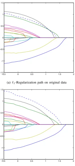
to explore how the ordering of the variables within the regularization path change as uncertainty is added. We first show a simple synthetic example there are
n = 100 samples in each class with x ∈ Rp, p = 22, with x ∼ N(µy,Σ). The class centroids are given by µ+1 = [−12,13,−12,−12,−12,−21,0,· · · ,0]T and
µ−1 = [12,−13,0,· · ·,0,0,0,0,0]T. The structure of Σ
is block diagonal, where diagonal components {σii}pi=1 are
equal to one and the block structure affects only the variables
x1, x2, x3, x4, x5, x6, where the off-diagonal elements in this
block {σij}6j=1,j6=i are equal to 0.1. The other off-diagonal
elements have covariance of zero.
Figure 2(a) represents the`1-regularization path as a function
of log10λon the original data. In Figure 2(b),x3has been
per-turbed such thatx3←x3+δ3with−ρ≤δ3≤ρ, which leads
to a shift in the ordering within the regularization path under normal `1-LR. Using the perturbed data set and knowledge
thatρ= 0.1forx3and presented with interval uncertainty, the
`1-regularized robust logistic regression recovers the original
ordering of the variables (see Figure 2(c)).
B. Human Rhino Virus Gene Expression Data
Here we present numerical results on peripheral blood gene expression data set from a group of n = 20 patients inoculated with the Human Rhino Virus (HRV), the typical agent of the common cold [19]. Half of the patients responded with symptoms (y= +1) and the other half did not (y=−1). The original12,023 genes on the Affymetrix oligonucleotide microarray were reduced to p= 129 differentially expressed genes controlling for a 20% False Discovery Rate (FDR) using the same methodology as applied in ([20]). We will regularize both the robust binomial deviance and standard binomial deviance with an `1-penalty to control the sparsity
of the resulting model forcing many elements inβ to be zero. In this experiment there were approximately 20 microarray chips that were technical replicates. The technical replicates were used to estimate the interval uncertainty bounds using (14).
Since oligonucleotide microarray devices detect the presence of mRNA abundance by including thousands of different probe sets (short sequences) that bind to a particular mRNA molecule, produced from a specific gene, we will adopt interval uncertainty across thepgenes. The estimated interval uncertainty bounds, {ρˆi(α)}pi=1, were obtained from (14)
using the empirical CDF of the independent technical replicate data with linear interpolation between sampled data. The CDF in (14) was computed by (15) with each conditional CDF centered about their class dependent sample mean and equal class priors ˆP(Y = +1) = ˆP(Y = −1) = 1/2. Technical replicates are generated from the blood sample used to assess gene expression activity in the training data and thus, are commonly used to isolate the effect of measurement error. We explored the effect of interval uncertainty bounds resulting from quantiles of (14) at levels of
α = {0.25,0.50,0.75,0.95,0.99}. Figure 3 shows the
`1-regularization paths obtained by solving (11) on the
training data for different interval uncertainty (including no uncertainty corresponding to standard `1-LR) and illustrates
how robustness affects the ordering of the genes. We see from Figure 3(a) that the first gene to appear in the regularization path is the anti-viral defense gene RSAD2. RSAD2 persists at the first gene in the regularization path for α = {0,0.25,0.50,0.75} (latter three not shown) but disappears from the regularization path completely, along with a few other genes, in Figure 3(a), when α = {0.95,0.99}.
!!"# ! !"# $ $"# % !$"# !$ !!"# ! !"# $ $"# & & '()*+,(&$ '()*+,(&% '()*+,(&-'()*+,(&. '()*+,(&# '()*+,(&/ '()*+,(&0 '()*+,(&1 '()*+,(&2 '()*+,(&$! '()*+,(&$$ '()*+,(&$% '()*+,(&$-'()*+,(&$. '()*+,(&$# '()*+,(&$/ '()*+,(&$0 '()*+,(&$1 '()*+,(&$2 '()*+,(&%! '()*+,(&%$ '()*+,(&%%
(a)`1-Regularization path on original data
!!"# ! !"# $ $"# % !$"# !$ !!"# ! !"# $ $"# & & '()*+,(&$ '()*+,(&% '()*+,(&-'()*+,(&. '()*+,(&# '()*+,(&/ '()*+,(&0 '()*+,(&1 '()*+,(&2 '()*+,(&$! '()*+,(&$$ '()*+,(&$% '()*+,(&$-'()*+,(&$. '()*+,(&$# '()*+,(&$/ '()*+,(&$0 '()*+,(&$1 '()*+,(&$2 '()*+,(&%! '()*+,(&%$ '()*+,(&%%
(b)`1-Regularization path with bounded perturbations in x3andρ3= 0.1 !!"# ! !"# $ $"# % !$"# !$ !!"# ! !"# $ $"# & & '()*+,(&$ '()*+,(&% '()*+,(&-'()*+,(&. '()*+,(&# '()*+,(&/ '()*+,(&0 '()*+,(&1 '()*+,(&2 '()*+,(&$! '()*+,(&$$ '()*+,(&$% '()*+,(&$-'()*+,(&$. '()*+,(&$# '()*+,(&$/ '()*+,(&$0 '()*+,(&$1 '()*+,(&$2 '()*+,(&%! '()*+,(&%$ '()*+,(&%%
(c)`1-Robust regularization path withρ3= 0.1
Fig. 2. Regularization paths as a function of log10λ: robust recovers original
ordering after perturbation
The three “robust genes” that persist across all explored values of αare ADI1, OAS1, and TUBB2A. Of these three, OAS1 (codes for proteins involved in the innate immune
response to viral infection) barely appears in Figure 3(a), yet is the first gene to appear in the robust regularization paths that is common to both α = {0.95,0.99} (see Figures 3(b) and 3(c)). These results suggest that when assessing variable importance via regularization paths, one should be aware of the effect of measurement uncertainty on the ordering of the variables.
The robust formulation within this paper aims at minimizing the worst-case configuration of perturbations on the logistic regression loss function. As our goal is discriminating between two phenotypes, it is of interest to compare the worst-case probability of error for LR and RLR on perturbed data sets, i.e.,xi←xi+δi,|δi| ≤ρˆi(α), after training on the original data. The`1-tuning parameter λfor both standard `1-LR and
`1-RLR was chosen to minimize the out-of sample probability
of error via 5-fold cross validation. Given the cross validated value of λ for both methods, the models were then fit to the entire set of training data. 50,000 perturbed data matrices were then generated subject to interval uncertainty bounds {ρˆi(α)}ip=1 for α = {0.25,0.50,0.75,0.95,0.99}. The
best-case and worst-best-case probability of error were recorded in Table I. We see for all values of α explored, the worst-case probability of error corresponding to `1-RLR is always less
than or equal to that of `1-LR. Whenα ={0.95,0.99}, the
worst-case probability of error for`1-LR is0.30but reduces to
0.20 when using`1-RLR with interval uncertainty estimated
from the data using (14). Corresponding to the worst-case probability of errors are the sensitivity and 1-specificity, given in Table II. We see that `1-RLR achieves the same power
as `1-LR at false alarm rates less than or equal to that of
the non-robust method. The proposed method can be used to reduce classifier error sensitivity in large scale classification problems. This can be important in practical applications such as biomarker discovery and predictive health and disease.
TABLE I
BEST AND WORST CASE PROBABILITY OF ERROR,Pe,FOR THEHRVDATA SET
α `1-LR `1-Robust LR
minPe maxPe minPe maxPe
0.25 0.10 0.15 0.10 0.15 0.50 0.05 0.20 0.10 0.20 0.75 0.10 0.25 0.10 0.25 0.95 0.00 0.30 0.05 0.20 0.99 0.00 0.30 0.00 0.20 VIII. CONCLUSION
Building on the results of [7] and [5], we have formulated the robust logistic regression problem with group structured uncertainty sets. By adding regularization penalties, one can enforce block-sparsity assumptions of the underlying signal. We have presented a block co-ordinate gradient method with iterative grouped thresholding for solving the penalized RLR problems. The group thresholding is affected by both the group-lasso penalty and the magnitude of the worst-case un-certainty. Thus, RLR tends to promote thresholding of highly
!! !" !# !$ % !& !' !! !" !# !$ % $ # " ()*$%+!,!-./0 123$ 445" 463"7$ 89:8# :1;$ <=17> 5;12# ;?5<3@?# AB>>#1 =@@$ (a)α= 0 !! !" !# !$ % !# !$&' !$ !%&' % %&' $ $&' # ()* $%+!,!-./0 123$ 456#7%$% 518$ 9:;:$<7= 9>==#1 (b)α= 0.95 !! !" !# !$ % !$&' !$ !%&' % %&' $ $&' ()* $%+!,!-./0 123$ 245'6 789:# ;1<$ <3=:>8$ ?@AA#1 (c)α= 0.99
Fig. 3. Regularization paths on the HRV data set as a function of log10λ/λmaxfor different magnitudes of interval uncertainty, as determined
by theαquantile
uncertain variables, essentially performing an initial step of variable selection. We have proposed an empirical approach to estimating the uncertainty magnitude using quantiles. This
TABLE II
SENSITIVITY AND1-SPECIFICITY CORRESPONDING TO WORST CASE PROBABILITY OF ERROR FROMHRVDATA
α `1-LR `1-Robust LR
Sens. 1-Spec. Sens. 1-Spec. 0.25 0.70 0.00 0.70 0.00 0.50 0.70 0.10 0.70 0.10 0.75 0.70 0.20 0.70 0.20 0.95 0.70 0.20 0.70 0.10 0.99 0.70 0.30 0.70 0.10
approach was applied to a real gene expression data set where quantile estimation was applied to a set of technical replicates. The numerical results on this data set establish that the proposed approach can yield lower worst-case probability of error and lower false alarm rates. Such a gain in worst-case detection performance can improve the performance for predictive health and disease, and in particular for predicting patient phenotype. It will be interesting to explore the situation when the group-structure of the uncertainty differs from that of the regularization penalty. This situation could potentially be solved by modifying the sparse group-lasso solution as in [21]. It is also of interest to explore the kernelization of this method in which one can study the propagation of bounded data uncertainty in a reproducing kernel Hilbert space.
ACKNOWLEDGMENT
The authors sincerely appreciate the thoughtful insight of Ami Wiesel in developing the ideas presented in this paper. The authors also appreciate the valuable suggestions made by Ji Zhu, Kerby Shedden, and Clayton Scott.
The views, opinions, and/or findings contained in this article/presentation are those of the author/presenter and should not be interpreted as representing the official views or policies, either expressed or implied, of the Defense Advanced Research Projects Agency or the Department of Defense.
”A” (Approved for Public Release, Distribution Unlimited) REFERENCES
[1] A. Wiesel, Y.C. Eldar, and A. Yeredor, “Linear regression with Gaussian model uncertainty: Algorithms and bounds,” IEEE Transactions on Signal Processing, vol. 56, no. 6, pp. 2194–2205, 2008.
[2] A. Wiesel, Y.C. Eldar, and A. Beck, “Maximum likelihood estimation in linear models with a Gaussian model matrix,” IEEE Signal Processing Letters, vol. 13, no. 5, pp. 292, 2006.
[3] R.J. Carroll, C.H. Spiegelman, K.K.G. Lan, K.T. Bailey, and R.D. Ab-bott, “On errors-in-variables for binary regression models,”Biometrika, vol. 71, no. 1, pp. 19–25, 1984.
[4] Sabine Van Huffel, Ivan Markovsky, Richard J. Vaccaro, and Torsten S¨oderstr¨om, “Total least squares and errors-in-variables modeling.,” Signal Processing, vol. 2007, 2007.
[5] S. Chandrasekaran, G. H. Golub, M. Gu, and A. H. Sayed, “Parameter estimation in the presence of bounded data uncertainties,” SIAM J. Matrix Anal. Appl., vol. 19, no. 1, pp. 235–252, 1998.
[6] Laurent El Ghaoui and Herv´e Lebret, “Robust solutions to least-squares problems with uncertain data,”SIAM J. Matrix Anal. Appl., vol. 18, no. 4, pp. 1035–1064, 1997.
[7] Laurent El Ghaoui, Gert R. G. Lanckriet, and Georges Natsoulis, “Robust classification with interval data,” Tech. Rep. UCB/CSD-03-1279, EECS Department, University of California, Berkeley, Oct 2003. [8] Gert R. G. Lanckriet, Laurent E Ghaoui, Chiranjib Bhattacharyya, and Michael I. Jordan, “A robust minimax approach to classification,” Journal of Machine Learning Research, vol. 3, 2002.
[9] Seung-Jean Kim, Alessandro Magnani, and Stephen P. Boyd, “Robust fisher discriminant analysis,” in In Advances in Neural Information Processing Systems. 2006, MIT Press.
[10] Huan Xu, Shie Mannor, and Constantine Caramanis, “Robustness, risk, and regularization in support vector machines,” CoRR, vol. abs/0803.3490, 2008.
[11] Aharon Ben-Tal, Laurent E. Ghaoui, and Arkadi Nemirovski, Robust Optimization (Princeton Series in Applied Mathematics), Princeton University Press, 2009.
[12] Ming Yuan, Ming Yuan, Yi Lin, and Yi Lin, “Model selection and estimation in regression with grouped variables,” Journal of the Royal Statistical Society, Series B, vol. 68, pp. 49–67, 2006.
[13] Lukas Meier, Sara van de Geer, and Peter B¨uhlmann, “The group lasso for logistic regression,”Journal Of The Royal Statistical Society Series B, vol. 70, no. 1, pp. 53–71, 2008.
[14] Dimitri P. Bertsekas,Nonlinear Programming, Athena Scientific, 1999. [15] Volker Roth and Bernd Fischer, “The group-lasso for generalized linear models: uniqueness of solutions and efficient algorithms,” inICML ’08: Proceedings of the 25th international conference on Machine learning, 2008, pp. 848–855.
[16] Stephen Boyd and Lieven Vandenberghe, Convex Optimization, Cam-bridge University Press, 2004.
[17] Jie Peng, Pei Wang, Nengfeng Zhou, and Ji Zhu, “Partial correlation estimation by joint sparse regression models,”Journal of the American Statistical Association, vol. 104, no. 486, pp. 735–746, 2009. [18] A. Wiesel, Y.C. Eldar, and S. Shamai, “Optimization of the mimo
compound capacity,” IEEE Transactions on Wireless Communications, vol. 6, no. 3, pp. 1094, 2007.
[19] A.K. Zaas, M. Chen, J. Varkey, T. Veldman, A.O. Hero, J. Lucas, Y. Huang, R. Turner, A. Gilbert, R. Lambkin-Williams, et al., “Gene Expression Signatures Diagnose Influenza and Other Symptomatic Res-piratory Viral Infections in Humans,”Cell Host & Microbe, vol. 6, no. 3, pp. 207–217, 2009.
[20] A. Swaroop, A.J. Mears, G. Fleury, and A.O. Hero, “Multicriteria Gene Screening for Analysis of Differential Expression with DNA Microarrays,” EURASIP Journal on Advances in Signal Processing, 2004.
[21] J. Friedman, T. Hastie, and R. Tibshirani, “A note on the group lasso and a sparse group lasso,” arXiv:1001.0736v1, 2010.