University of Warwick institutional repository: http://go.warwick.ac.uk/wrap
This paper is made available online in accordance with
publisher policies. Please scroll down to view the document
itself. Please refer to the repository record for this item and our
policy information available from the repository home page for
further information.
To see the final version of this paper please visit the publisher’s website
.
Access to the published version may require a subscription.
Author(s): K Hemming and JL Hutton
Article Title: Sensitivity Models for Missing Covariates in the Analysis
of Survival Data from Multiple Surveys
Year of publication: 2007
Link to published article:
http://www2.warwick.ac.uk/fac/sci/statistics/crism/research/2007/paper
07-12
Sensitivity models for missing covariates in the
analy-sis of survival data from multiple surveys
K. Hemming J. L. Hutton
Department of Statistics, University of Warwick.
Summary. Using individual patient data from five independent surveys, we evaluate regional variations in survival in cerebral palsy. The influence of four important variables measuring dis-ability, which are only partially observed for many cases, are analysed. Results are compared between a naive complete case analysis; a full likelihood model in which the covariates are assumed to be missing at random and in which each of the binary predictor variables are mod-elled as independent Bernoulli random variables; a model in which the covariates are modmod-elled by a conditional wise sequence, accommodating dependencies between the likelihoods of hav-ing various mixtures of disabilities; and a model in which the likelihood of a predictor variable being observed is allowed to depend on the value of the covariate itself (NMAR). Fully para-metric survival regression models are used and analysis carried out in BUGS. Results suggest that proportions recorded as having severe visual or cognitive impairments are substantially lower than the actual proportions severely impaired. Associations between the likelihood of a particular covariate being recorded and the likelihood of a more severe disability imply that life expectancies for those who are very severely impaired may be up to20%less than inferences based on complete case analyses.
Introduction
Cerebral palsy is a common cause of childhood disability, affecting both physical and men-tal abilities. Survival is known to be affected by severity of impairment, measured by such factors as severity of manual and ambulatory functions, severity of cognitive, visual and hearing abilities (Evans et al. (1990); Hutton et al. (2000); Hutton and Pharoah (2002); Hemming et al. (2006)). Estimates of life expectancies in cerebral palsy are important for effective planning of resources and knowledge of levels of care which will be required in the future. Life expectancies also play an important role in medico-legal settlements. Indirect comparisons between different regions and countries, from published survival studies, ap-peared to suggest that there may be some variation between life expectancies for those with cerebral palsy (Hutton et al., 2000). For example, of those with a severe manual disability, 47% were reported to survive to age 30 years for the Mersey Cerebral Palsy Register, com-pared to 60% for the North of England Collaborative Cerebral Palsy survey (Hutton et al., 2000).
regions due to a particularly high proportion of missing data (63% for one covariate). It is a real concern that those who are very severely impaired may die before assessments of severity have been carried out, and they may therefore not be representative of the sample as a whole, thereby not meeting the underlying assumption of a complete case analysis, that of the data being missing completely at random. It is our aim here to consider how sensitive questions of regional variation in survival and estimates of life expectancies are to various patterns and assumptions of the missing covariate data.
Inferences for life expectancies in cerebral palsy from multiple data sources
In the UK there are five cerebral palsy registers, each covering a separate (although non exhaustive), region of the UK, comprising the Mersey region, the North of England, the Ox-ford region, Northern Ireland and Scotland. Each of these five registers have independently carried out retrospective surveys or have prospectively collected information on those born with cerebral palsy to mothers resident within defined geographical regions over various time periods. Furthermore, each register also flags all cases with the national births and deaths registers (the National Health Service Central Register for England, the Northern Ireland Central Services Agency or the General Register Office for Scotland). All individuals having been identified as having cerebral palsy from each of these five regions are represented using anonymised data on the collaborative UKCP database. The database therefore comprises a well defined cohort of people with cerebral palsy, for virtually all of whom vital status information is known.
Survival predictions as a function of severity of impairment are dependent on knowledge of the severity of the impairment. The severity of impairments is usually evaluated between the ages of two and five years. For children who die before an evaluation is made, information on severity of impairment may be missing. This covariate data can also be missing for those children who are still alive, perhaps because the child moved out of the region or was lost to follow-up (for covariate information and not death information, which are distinct processes) for some other reason. The proportions of cases with missing information on severity vary between the five regions, with some having high levels of recorded data, whilst others having high proportions of missing data.
Missing covariate data in survival analysis
Following standard notation, we use capital letters to denote random variables, lower case letters to denote realisations of random variables and distinguishing vectors using bold type face for realisations of random variables and for parameters. LetY = (Y1, . . . , YP), with realisationy, be aP dimensional vector representing complete data onP variables. LetRp (p= 1, . . . , P) be an indicator for whether variableYpis observed, so thatR= (R1, . . . , RP) is a vector of observed data indicators, with realisationrand with density functionfR(r;ψ). Without loss of generality, let Y, with density function fY(y;θ), be partitioned into an observed and missing part,Y = (Yo, Ym) whereYois the observed component ofY andYm the missing component ofY.
Following Rubin’s terminology (Rubin, 2002), the data are said to be Missing Completely At Random (MCAR) if:
that is the missing data mechanism does not depend on either the observed (Yo) or missing data (Ym). A Complete Case Analysis (CCA), that is deleting or ignoring, any observations with incomplete or missing data, will only result in unbiased estimates where the data are MCAR. Even when data are MCAR estimates may be inefficient if large numbers of observations are excluded. Where the data are not MCAR, a CCA leads both to reduced efficiency and possible biased estimates of covariate effects.
Data are said to be Missing At Random (MAR) if:
fR|Yo,Ym(r|yo,ym;ψ) =fR|Yo(r|yo;ψ) (2)
that is, the data are missing in a way that is MCAR after conditioning on other observed data. MAR is therefore a less restrictive assumption than to MCAR.
Under likelihood based inferences, the observed data are (Yo, R) and the likelihood of interest for this observed data isL(θ|Yo, R), such that:
L(θ|Yo, R) ∝ fYo,R(yo,r;θ,ψ)
= Z
Ym
f(Yo,Ym,R)(yo,ym,r;θ,ψ)dYm
= Z
Ym
fR|Yo,Ym(r|yo,ym;ψ)fYo,Ym(yo,ym;θ)dYm. (3)
This likelihood is intractable unless either a full specification of the missing data mechanism, fR|Yo,Ym(r|yo,ym;ψ), is given, or if fR|Yo,Ym(r|yo,ym;ψ) = fR|Yo(r|yo;ψ). Under this
simplification the likelihood reduces to:
L(θ|Yo, R) ∝
Z
Ym
fR|Yo,Ym(r|yo,ym;ψ)fYo,Ym(yo,ym;θ)dYm
= fR|Yo(r|yo;ψ)
Z
Ym
fYo,Ym(yo,ym;θ)dYm
∝
Z
Ym
fYo,Ym(yo,ym;θ)dYm
= fYo(yo;θ)
∝ L(θ|Yo). (4)
This simplification holds when the data are MAR, andθandψare distinct, or for Bayesian inferences are a priori independent. The missing data mechanism is then said to be “ignor-able”, since inferences can be made from the likelihood of the observed data,L(θ|Yo).
case analysis method is the routine and in many cases only survival method available in statistical packages. Likelihood based inferences for MAR covariates require the model is parameterised in terms of the conditional density function forT,fT|Z(t|z;θT|Z), and the
marginal density for Z, fZ(z|θZ) where θ = (θT,θZ) represents the parameters for the
survival distribution and covariate distribution functions respectively (Lipsitz and Ibrahim, 1996a). WritingZ = (Zo, Zm), so thatYo = (T, δ, Zo), for the case in whichZ is MAR, likelihood based inferences reduce to:
L(θ|Yo) ∝ fYo(yo;θ)
= fT,δ,Zo(t, δ,zo;θ)
= fT,δ|Zo(t, δ|zo;θT)fZo(zo;θZ) (5)
(6)
that is, specification of both fT|Z(t|z,θT), of main interest, and fZ(z;θz), often of lesser
interest, are required.
For the Cox proportional hazards survival model methods have been developed to accom-modate missing at random categorical or continuous covariate data (Herring and Ibrahim (2001); Herring et al. (2002); Chen et al. (2002)), as have methods for parametric survival models (Lipsitz and Ibrahim (1996a); Schluchter and Jackson (1989); Lipsitz and Ibrahim (1996b); Meng and Schenker (1999); Cho and Schenker (1999)). Of these, two have consisted of Bayesian approaches: a piecewise constant proportional hazards cure rate model (Chen et al., 2002); and a log-F accelerated failure time model for missing at random categorical and continuous covariates (Cho and Schenker, 1999).
Where the MAR assumption does not hold, the data are said to be Not Missing At Random (NMAR) and the missing data mechanism said to be “non-ignorable”. In this situation the mechanism for the missing data, that is fR|Yo,Ym(r|yo,ym;ψ), must also
be specified and included in likelihood inferences (equation 3). Since (Yo, Ym, R) is not observed in full, this may lead to issues of identifiability forfR|Yo,Ym(r|yo,ym;ψ) (Baker
and Laird, 1988). Within the remit of generalised linear models, non-ignorable missing data mechanisms have been modeled (Ibrahim et al., 1999; Stubbendick and Ibrahim, 2003), and Bayesian approaches have used informative priors to identify model parameters with NMAR covariates (Huang et al., 2005). In survival analysis, within a proportional hazards cure rate model, non-ignorable models have been proposed using maximum likelihood based techniques (Herring and Ibrahim, 2002).
Existing methods for dealing with missing covariate data in survival analysis, both Bayesian and frequentist, are often not easy useable by others and so have limited practical applicability due to computational programming required. Furthermore, to our knowledge there have been no Bayesian developments of survival regression models for non-ignorable missing data mechanisms. The accelerated failure time models are a wide class of log-linear models which provide an alternative to the Cox model when assumptions of proportionality are not met, and being fully parametric they can also be more powerful. The accelerated failure time models have also been shown to fit the UKCP data well (Kwong and Hutton, 2003) and may be more robust in cases of model mispecification (Hutton and Monoghan, 2002).
extensions to covariate data not missing at random, and consider how robust estimates are to various non-ignorable missing data mechanisms supported by the data. Although specified in terms of impairment variables and regional effects, the model is more generally a log-normal survival model for multiple and partially observed binary covariates with extra variation due to center, region, or other familial variable (or some other fully observed categorical covariate). Extensions included allow for interactions between the covariates and the inclusion of fully observed continuous covariates.
This paper is organised as follows. In the next section the fully parametric Bayesian survival model is outlined and models for the covariate data proposed. Likelihood based methods using Markov Chain Monte Carlo (MCMC) simulations are used to draw param-eter inferences under the less restrictive assumption of MAR. A parametric distribution is specified for the missing data mechanism, that is the likelihood of a covariate being ob-served, with dependencies on censoring status, survival time, and the covariate itself. Using weakly informative priors, we obtain posterior parameter estimates and consider how sen-sitive model inferences are to possible non-missing at random missing data mechanisms. In the final section, the model is applied to the UKCP data and inferences drawn. We compare inferences from a naive CCA to the better fitting models under a MAR analysis, and consider how robust parameter inferences are under possible NMAR mechanisms. The BUGS code for this model is available from the first author on request.
Proposed model
Survival distribution Let T have density function fT|Z(t|z;θT) conditional on binary
covariates z = (z1, . . . , zk). Full data, for individuals i = 1, . . . , nj, out of j = 1, . . . , J regions, are observed for event timestij and censoring indicatorsδij. The binary covariate data onzij= (z1ij, . . . , zKij) are only partially observed. Letyij = lntij. LetST|Z(t|z;θT)
andhT|Z(t|z;θT) represent the corresponding survival and hazard functions respectively.
We initially assume that there is an underlying effect of severity of impairment on survival across all five regions. We allow the survival to differ between the regions, in addition to that which might be explained by random variation. We therefore propose a model which allows for extra regional variation:
ln tij =α0+αzij+b(s)j+ση where η∼N[0,1] (7)
and whereb(s)j is a fixed effect due to region. We use the notationb(s)j(forj= 1, . . . , J−1) to refer to a regional effect (j) on survival (s) - as opposed to regional effects on proportions impaired (to be introduced later). We focus on the log-normal survival model and consider generalisablity to other distributions in the discussion. The resulting model is the log-normal survival model, withα0the intercept parameter,αrepresenting the set of covariate effects,
b(s) = (b(s)1, . . . , b(s)J−1) a set of regional effects on survival and σ the scale parameter, withθT = (α0,α, σ,b(s)).
Regional variation in the survival of both the severely impaired and non severely im-paired is incorporated by including an interaction between regions and the binary covariates:
lntij=α0+αzij+cjzij+b(s)j+ση (8)
Incorporating additional fully observed covariates (˜z) is straightforward:
lntij =α0+αzij+d˜z+b(s)j+ση (9)
where d represents the effect of a fully observed vector of continuous covariates (˜z), and θT = (α0,α, σ,b(s),d).
Covariate distributionLetz= (z1, . . . , zK), the indicators of severity of impairment
forK binary covariates (where 1 represents a severe impairment) have probability distri-butionfZ(z;θZ).
Since inferences for the covariates are not a prime interest of the analysis, one approach is to base inferences on a simple Bernoulli distribution of the form:
zk∼Bern(pk) (10)
wherepk represents the probability of a severe impairment for each of theKcovariates and where each of the variableszk are independently distributed binary variables:
fZ(z;θZ) = K Y
k=1
fZk(zk;pk) (11)
where θZ = (p1, . . . , pK). This implies that the probability of having a particular severe impairment is independent of any other severe impairments. This is not necessarily a valid assumption, but one which is investigated since it greatly reduces the computational time, as there are onlyK nuisance parameters.
An alternative is to specify the joint distribution forfZ(z;θZ) by a series of conditional
distributions (Lipsitz and Ibrahim (1996b); Ibrahim et al. (1999)):
fZ(z;θZ) =
1 Y
k=K
fZk|Z1:Zk−1(zk|z1:zk−1;βk) (12)
where θZ = (β1, . . . ,βK). In this way, correlations are induced between likelihoods of
each severe impairment, in contrast to the independent specification of probabilities in equation 11. For example, in the case of four covariates:
fZ(z;θZ) = fZ4|Z1:Z3(z4|z1:z3;β4)fZ3|Z1:Z2(z3|z1:z2;β3)fZ2|Z1(z2|z1;β2)fZ1|(z1;β(13)1).
Each conditional distribution may be represented by a logistic relationship. That is, the conditional probability of having a particular severe impairment, given a subset of other impairments, is modeled as a linear combination of this subset on the logit scale:
logit ˜pk=βk0+βk1z1+. . .+βkk−1zk−1 (14)
To allow the conditional proportion ( ˜pk) of those severely impaired to be similar between the regions, with some variability due to extra variation between the regions, a fixed regional effect can be incorporated:
logit ˜pk=βk0+βk1z1+. . .+βkk−1zk−1+b( ˜p)kj (15)
where b( ˜p)kj represents a fixed regional effect in (conditional) proportions ( ˜pk) severely impaired. Under this conditional wise specification with regional variations in proportions severely impaired,θz= (β1, . . . ,βK,b(p˜)1, . . . ,b(˜p)K), whereb(p˜)k = (b( ˜p)k1, . . . , b( ˜p)kJ−1).
Sensitivity analysis (NMAR extension)The covariate data are not fully observed,
and this is represented using a missing data indicator,rkij, such that:
rkij = 1 if covariatekis observed for individualiin regionj (16) = 0 otherwise.
Where the covariate data are not missing at random, likelihood based inferences require full specification of the missing data mechanismfR(r;ψ), which is here modeled as a logstic function:
logitp(r)kij =γk0+γk1zijk (17)
wherep(r)kij represents the probability of covariatekbeing observed for individual ifrom regionj. Here the probability that a covariate is observed depends only on the covariate value itself, withψ= (ψ1, . . . ,ψK) and where ψk= (γk0, γk1).
The probability of observing a particular covariate may depend on event time and, or censoring status. Where the missing data mechanism is allowed to depend on the cen-soring status, the independent cencen-soring assumption is replaced by independent cencen-soring conditional onR(Rathouz, 2007).
logitp(r)kij =γk0+γk1zijk+γk2tij+γk3δij. (18)
So thatfRk(rk;ψk) follows a logistic distribution with parameterψk = (γk0, γk1, γk2, γk3) andψ= (ψ1, . . . ,ψK). Regional effects on the missing data mechanism are not considered as this would require a large number of additonal parameters.
Likelihood Inferences
All inferences are carried out in BUGs using Markov Chain Monte Carlo methods, and models compared using DIC (Spiegelhalter et al., 2002). For completeness the likelihood is presented.
Inferences ignoring the missing data mechanism lead to L(θ|t,δ,z,r) ∝ L(θ|t,δ,z), wheret= (t1, . . . , tn),δ= (δ1, . . . , δn),r= (r1, . . . ,rn) and the parameter of interest isθT
and nuisance parameterθZ. The full likelihood is based on the factorisation of the joint
distribution forfT,δ,Z(t, δ,z;θ) =fT,δ|Z(t, δ|z;θT)fZ(z;θZ) so that:
L(θ|t,δ,z) ∝
N Y
j=1 nj Y
i=1
Wherezij is fully observed:
lij = ST|Z(tij|zij;θT)hT|Z(tij|zij;θT)δijfZ(zij;θZ). (20)
Wherezijis only partially observed, letG= 2K represent the number of possible
combina-tions of covariates (from now on called groups), with associated covariatezg(g= 1, . . . , G),
being one realisation of the G possible combinations of z. Let Wgij be an indicator for whether the partial observed covariate information on individualifrom regionj is compat-ible with the realisationzg, then:
lij = G X
g=1
WgijST|Z(tij|zg;θT)hT|Z(tij|zg;θT)δijfZ(zg;θZ). (21)
For non-ignorable missing data mechanisms:
L(θ,ψ|t,δ,Z,r) = N Y
j=1 nj Y
i=1
lij, (22)
where forzij only partially observed:
lij = G X
g=1
WgijST|Z(tij|zg;θT)hT|Z(tij|zg;θT)δijfZ(zg;θZ)fR|T,Z(rij|tij, δij,zg;ψ).(23)
As the data (T, δ, Z, R) are not fully observed (sinceZis only partially observed), it may not be possible to identify the parametersψ in fR(r;ψ). No algebraic check of identifiablity has been established, but in other similar models, using weakly informative priors, the parameter ψ has been identifiable (Huang et al., 2005). Non-identifiability in practical applications generally manifests as divergence or slow mixing of chains. Furthermore, even for an identifiable model, there is clearly no means of evaluating distributional assumptions for the missing data mechanism. Following others we therefore propose to use posterior inferences for (θT,θZ) based on weakly informative priors forψ, in the role of a sensitivity
analysis, to investigate how robust and sensitive inferences are to departures from the assumption of MAR.
Application
z-score values (around -3) indicate that the child was born with a very low birthweight for gestation, and values around zero suggest an average birthweight. Birthweight and gestational age are routinely recorded neonatal variables and are fully observed for this data set and so z-scores are derivable for the entire data set. This variable is of particular interest in current epidemiological research in cerebral palsy (Jarvis et al. (2003); Hemming et al. (2007)).
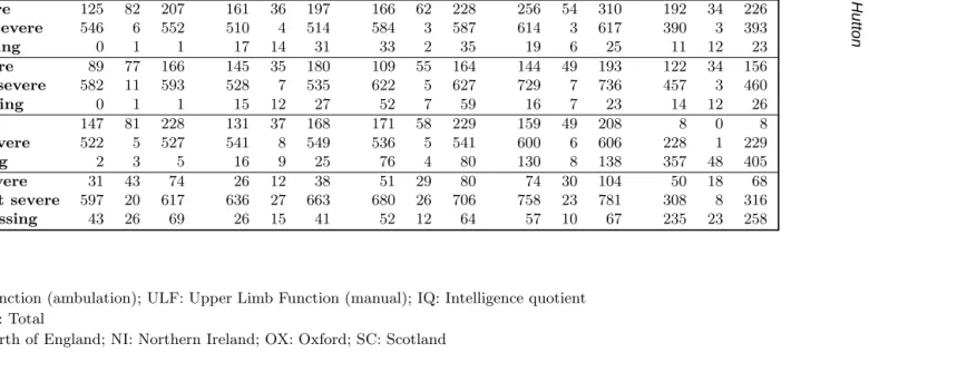
Proportions of cases with a particular severe impairment vary quite considerably between the regions (Table 1). Scotland stands out as the most noticeable extreme. Proportions of cases for which information on severity of impairment is missing, varies both between the regions and between the variables (Table 1). For manual and ambulatory severity indicators, the proportions of cases for which the severity indictor is missing, is low (less than 10%). For the other associate impairments, proportions of missing data are higher, for both Northern Ireland and Oxford, and very high for Scotland (63% with missing IQ information). The vast majority of cases have covariate information on at least one variable, with many having information on two or three covariates: 2980 (76%) have full covariate information on four covariates; 661 have data on three covariates; 226 have data on two covariates; 26 have data on one covariate only; 53 cases have no information on any of the four covariates.
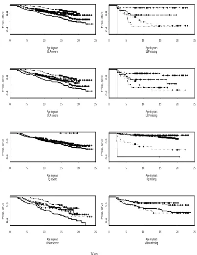
Some association between severity of disability and missing information may be due to the child having died before the assessment could be made or through lack of follow-up (for covariate data rather than death information). The Kaplan-Meier estimates of the survival by region and severity or missingness of impairment variables indicate there are many likely causes of missing covariate information (Figure 1). For example, for both manual and ambulatory variables for Mersey, missing data show a strong association with early deaths, although the absolute number of cases with missing information on these two variables for the Mersey region is small. In the North of England, Oxford and Scotland those with missing covariate information on ambulatory and manual variables constitute a mixture of early deaths and late censored observations, contrasting with Northern Ireland in which almost all those with missing information on these two variables are late censored observations. For those with missing cognitive impairment, again Mersey constitutes mainly deaths, and the North of England a mixture of early deaths and late censored observations, for Northern Ireland and Oxford, the missing covariate observations consist of mainly censored survival times. In Scotland, where the proportion of cases with missing information on severity of cognitive impairment is high, a significant proportion of those with missing cognitive data have died. For those with missing visual impairment, a large number of early deaths give a survival pattern which is not too dissimilar to those who are severely impaired for all five regions.
Implementation
We compare inferences from a complete case analysis where it is assumed the covariate data are MCAR, to inferences obtained under the less restrictive assumption of MAR and where to enable likelihood based inferences, not only fT|Z(t,z;θT) is modeled (for which
we consider models 7-9), but so too isfZ(z;θZ) (for which we consider models 10-11 and
12-15). We further consider how robust parameter estimates are to non-missing at random missing data mechanisms (models 17-18).
that this set of parameters are robust to prior specification). These parameters consist of the regression coefficients (α0,α,c,d), for which we used diffuse independent normal priors N(0,0.001) - (parameterised by center and precision parameters); the scale parameter,σa Gamma prior G(1,0.001) (approaching a uniform prior over the range (0,100) on the preci-sion scale); for the covariates (Bernoulli specification), non-informative Beta priors B(1,1) forpk and for the conditional wise specification, independent normal priors N(0,0.001) for βkk.
Inferences might be less robust to priors for the parameters of the missing data mech-anism fR(r;ψ). For these parameters we considered various weakly informative priors: N(0,0.1), a fairly tight prior centered around zero; N(0,0.01) a more uniform prior again centered at zero; N(0,0.001) towards a vague prior again centered at zero.
All inferences were carried out in BUGS (Spiegelhalter et al., 1999) with convergence checked using CODA (Best et al., 1997). All inferences were compared over 100,000 iter-ations after an initial burn in of 10,000 iteriter-ations. A diffuse range of starting values were explored. For missing binary covariate data, zero and one values were randomly imputed to generate a set of initial covariate values. Model fits were compared using deviances with complexity penalised by twice the number of parameters, along the lines of DIC. The or-der of the conditional specification forfZ(z) was chosen by the order providing the lowest DIC value, although the main parameters of interest were not sensitive to choice of order. The order used wasz1=ambulatory impairment;z2=manual impairment;z3=cognitive im-pairment;z4=visual impairment. No interactions were found to be significant and are not presented.
Sample run times for this fairly large data set (n=3946) were for the CCA 107 seconds; for the MAR analysis with independent Bernoulli model forfZ(z|θz) 206 seconds; for the
MAR analysis with conditional model forfZ(z|θz) 1076 seconds; and for the NMAR model
21708 seconds.
Results
Inferences from a CCA
As expected, in a CCA the distribution assigned tofZ(z;θz) has no impact on any survival
analysis inferences (as is demonstrated in Table 2). Inferences for fT|Z(t,z;θT) allowing
dependencies on the four binary predictor variables and with extra variation due to region (modeled as in equation 7), suggests that out of the four predictive covariates, a severe ambulatory impairment reduces the median life time by the most (Table 2). Furthermore, a regional variation in survival is significant, with Scotland seemingly having a much more favorable outlook compared to the other four regions (coefficient 26(11.98)). Clearly since Scotland has such high proportions of missing sensory data, such a conclusion is questionable under anything but a completely naive CCA.
Inferences from a MAR analysis
Using a MAR likelihood based approach it is necessary to modelfZ(z;θZ). Although
attrac-tive, a simple independent parameterisation for fZ(z;θZ) through independent Bernoulli
also results in smaller standard errors on parameter estimates compared to the model in which the Bernoulli specification is used (Table 2).
Using an independent Bernoulli model for fZ(z;θZ), a MAR analysis finds only a
marginally significant difference between the five regions in survival: deviance of 20590 (no region effect - 10 parameters) vs 20580 (with region effect - 14 parameters) (Table 2). Contrasting this, under the conditional specification forfZ(z;θZ), a significant difference
between Scotland and the other four regions persists under the MAR fit, with Scotland again standing out as having the most favorable outlook ( deviance of 15820 (no region effect - 16 parameters) vs 15790 (with region effect 20 parameters)). Standard errors on fixed effect region parameters are smaller under the MAR fit compared to the CCA (this holds for both the conditional and Bernoulli models).
For models in which a regional effect on survival is included, under the Bernoulli specification for fZ(z;θZ), the effect of a severe ambulatory impairment decreases from −0.86(0.19) in a CCA to −1.08(0.28) in a MAR analysis (Table 2). This suggests a much greater reduction in life expectancies for those with a severe ambulatory impairment than previously thought (i.e. from inferences based on a CCA). However, using a conditional wise specification for fZ(z;θZ), the effect of a severe ambulatory impairment is −0.87(0.18),
very similar to that of the CCA, and with a much smaller standard error compared to the Bernoulli model for fZ(z;θZ). Using the conditional wise specification for fZ(z;θZ),
the reduction in life expectancy associated with the three severe impairments, ambulation, manual and cognitive disabilities are fairly similar, as opposed to the CCA where a se-vere ambulatory impairment appears to have the greatest impact on a reduction in life expectancy.
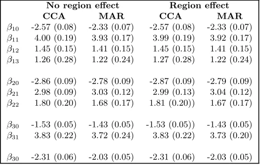
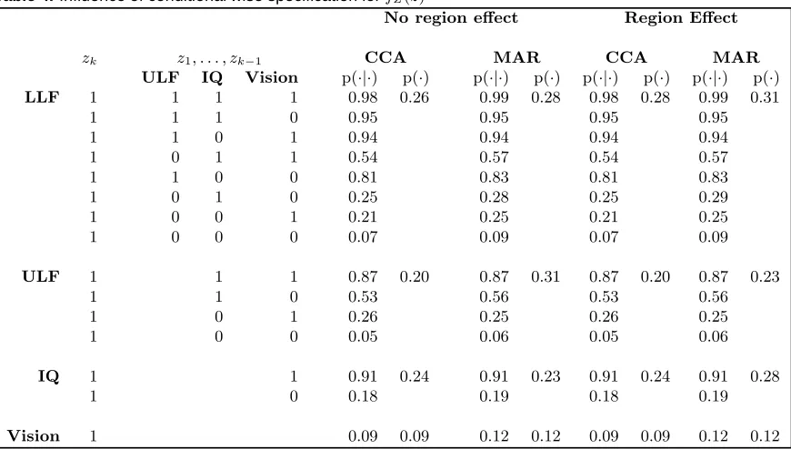
Parameter estimates for the parameters of less interest (those of fZk|Z1:Zk−1(zk|z1 : zk−1;βk)) are given in Table 3, and an interpretation of these parameter estimates in
Ta-ble 4. There is a strong correlation between a severe ambulatory impairment and the other three impairment variables: someone who has a severe ambulatory impairment has a very high likelihood of having a severe manual, visual or cognitive impairment (Table 4), with probabilities ranging from 0.81 to 0.98. A severe cognitive impairment is also highly corre-lated with a severe visual impairment, and having both a cognitive and visual impairment is highly correlated with a severe manual impairment.
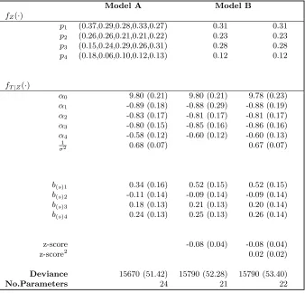
There is some regional variation in proportions severely impaired (Table 1). In a fur-ther attempt to improve model fit under MAR inferences, we consider a fixed regional effect on the proportion severely impaired, using a conditional specification forfZ(z;θz)
(equation 15). This model gives a lower deviance value compared to models in which no regional variation between proportions severely impaired are included (deviances 15760 (24 parameters) vs 15790 (20 parameters)). Posterior parameters indicate that there is no-ticeable regional variation in proportions of cases with each of the four severe impairments (Table 5). For instance, in Scotland, 37% are estimated to have a severe ambulatory impair-ment, compared to the 31% average over regions; only 6% in the North East are estimated to have a severe visual impairment (compared to the average of 12%, with as many as 18% in Scotland). Cognitive information has particularly high proportions of missing data in Scotland, with just 3% of those with known data on this variable having a severe impair-ment. MAR inferences estimates 15% of cases in Scotland as having a severe intellectual impairment, lower than the average (26%), but a vast improvement on 3%. Main parameter estimates forfT|Z(t|z;θT) do not differ greatly to those of previous MAR fits, except that
measured in terms of a deviation from expected birthweight for a given gestational age, called “z-scores”. This is a fully observed continuous covariate. Both linear and quadratic effects are investigated as this variable is thought to have an inverse J relationship with the incidence of cerebral palsy and so might be expected to affect survival outcome in a similar way. Neither models provided a significant improvement in model fit (Table 5). This is in contrast to the CCA (previously published (Hemming et al., 2005) and not shown here) where it was found to have a significant influence.
NMAR sensitivity analysis
We consider allowing the missing data mechanism to be non-ignorable, parameterised by a logistic function with dependencies on the event time, censoring status and covariate (equa-tions 17 and 18). We consider only the better fitting model for the covariate distribution, and all results presented on based on the full conditional wise specification (equation 14). Main parameter estimates were not sensitive to choice of prior and results presented are based on the priorN(0,0.01).
NMAR and MAR models are compared (Table 6) by fitting full NMAR models in which dependencies on time, censoring and covariate are included; with NMAR models in which only an intercept term is included in the distribution for the missing data mechanism (and so therefore reduces to a MAR model). The NMAR models provide a better fit, in terms of smaller deviances, than the NMAR models in which only the intercept term is included. This suggests the covariate data may be NMAR. As with MAR fits, a model in which region is included as a survival regression model appears to give a better fit. However, the extent to which the model is improved by including an effect due to region, both in terms of deviance and parameter estimates, is greater under the NMAR models. Under the better fitting NMAR model with variation due to region included, posterior estimates forαsuggest that the coefficients for the effects of both manual and ambulatory functions are similar (around -0.86); and coefficients for both cognitive and visual disabilities are also similar (around -0.7). Scotland again appears to have significantly better survival outcomes compared to the other four regions, and variation between the other four regions is similar to that of the MAR models.
Clinical conclusions
A naive CCA leads to conclusions of a regional variation in survival outcome, with estimated proportions severely impaired (26%,20%,24%,9%), with order of magnitude on survival influence: ambulation, intelligence, manual dexterity, and vision; and order of influence of region on survival: the North of England (worst), Mersey, Oxford, Northern Ireland, Scotland (best). Scotland having the best survival outcome, is however dubious under such a complete case analysis as Scotland has such high proportions of missing data.
A full and in depth analysis of this data involves fitting a more complex model to the like-lihood of a severe impairment, in which correlations between the four variables are induced (through a conditional wise specification), and this results in a better fitting model. Under such a MAR model fit, proportions severely impaired are higher (31%,23%,28%,12%), the effect of the covariates on survival similar between models in which an effect of region is included and one which is not, and interestingly, Scotland again comes out as having the best survival outcome. All three of ambulation, manual dexterity and intelligence, are es-timated to have similar affects on median life expectancies. This model leads to greater precision in main parameter inferences compared to the CCA, a reflection of the larger sample size and how the extra uncertainty introduced by the partial covariate information has been reduced by modeling correlations between each of the four impairments. A model in which the proportions of cases with each of the severe impairments are allowed to vary between the regions produces a slightly better fit. Under such a model the proportion of cases with a severe intellectual impairment in Scotland is estimated to be around 15%, which is much lower than the average over the regions, but substantially higher than the raw data for Scotland leads us to believe at just 3%. A sensitivity analysis, allowing for the covariate data to be missing in a non-random way, suggests a further increase in the proportions severely impaired, especially those with severe visual or cognitive impairments ((32%,24%,33%,16%)).
One of the primary questions of interest in the analysis of this data, is whether there exists a regional variation in survival. Such regional variations may possibly be due to such factors, as variations in neonatal care, variations in racial, ethnic or socio-economic mixes of the background populations of the regions, which may indirectly affect rates of cerebral palsy, rates of the severely impaired and survival outcomes. A CCA, conditioning on severity of impairment, suggests no regional variation between four (Mersey, North of England, Northern Ireland, Scotland) of the regions, but suggests an improvement in survival in Scotland. Our in depth MAR analysis, again suggests no regional variation between these four regions, but finds that survival in Scotland is significantly improved. This apparent favorable outlook in Scotland may reflect a true increase in life expectancy or may be an artifact of the data, since even an analysis with complete covariate data may be compromised by differing ascertainment proportions between the regions. Scotland has higher proportions severely impaired for all impairment variables except for cognitive impairment, which could suggest an under-ascertainment of the less severely impaired cases. Further analysis have shown estimated prevalence rates of cerebral palsy in Scotland to be significantly lower than those of the other four regions, a further indication of reduced ascertainment (personal communication, Jane Hutton).
conditional wise specification for the covariates, as 15.5 years (exp(6.69)/52); interestingly under the NMAR analysis this median life expectancy is similar (exp(6.70)/52), a reflection of those with missing covariate information being both deaths (providing a reduction in life expectancies) and censored observation (providing an increase in life expectancies). A CCA leads to the conclusion that ambulation provides the most predictive information for a reduction in life expectancy. Results here however suggest that the four severe impairment variables have similar predictive powers, a conclusion that has some clinical feasibility due to all four variables acting as surrogate markers for a degree of cerebral damage which is difficult to quantify.
The estimated proportion of cases with a severe visual impairment is high (around 16%) compared to less than 10% from the CCA. However, this pattern of informed missingness detected by the NMAR model, and the MAR model in which correlations between each of the impairments were included, would seem to be consistent with clinical expectations. Although in the UKCP no distinction is given to various types of missingness, in the Mersey region information is recorded on those with a possible visual impairment but one which is difficult to test (either because the child is too young or too severely impaired to test). For the Mersey region, 8% have “unknown” severity of visual impairment and an additional 12% fall into the group with a possible impairment, thereby suggesting that many more than the 8% have a severe visual impairment (Hutton and Pharoah, 2002). The NMAR analysis for the visual covariate, suggests a stronger association between the covariate being missing and the individual having died, than for the other three covariates.
Discussion
Missing covariate data often do not meet the assumption of being MCAR. The lesser re-strictive assumption of MAR is attractive, although when using likelihood based inferences requires additional assumptions for variables often of secondary interest, that of the covari-ate distributions in survival analysis. For a conceptually simple problem of relating survival outcome to four binary predictor variables with extra variation due to region or center and allowing for interactions and a fully observed continuous covariate, we have shown that careful consideration to the joint distribution for the covariates is a minimal requirement in meeting the MAR assumption. In our application the simple independent Bernoulli model for these four binary variables resulted in a poorer and misleading fit, than did a conditional wise specification for this joint density. This addresses in part the common concern of using independent prior distributions.
with an adaptive rejection sample. Our focus has been on binary covariates, which were of clinical interest in this example, though we have illustrated an extension to include a fully observed continuous covariate. Extensions to missing at random continuous covariates are a natural next extension, with incorporation into the conditional wise specifications, as too are informative Bayesian priors.
References
Baker, S. G. (1994). Regression analysis of grouped survival data with incomplete covariates: non-ignorable missing data and censoring mechanisms. Biometrics 50, 821–826.
Baker, S. G. and N. M. Laird (1988). Regression analysis for categorical variables with outcome subject to non-ignorable non response. Journal of the American Statistical Association 83, 62–69.
Best, N., M. K. Cowles, and K. Vines (1997). CODA: Convergence diagnostics and output analysis software for Gibbs sampling output, version 0.4. Downloadable from http://www.mrc-bsu.cam.ac.uk/bugs/.
Chen, M. H., J. G. Ibrahim, and S. R. Lipsitz (2002). Bayesian methods for missing covariates in cure rate models. Lifetime data analysis 8, 117–146.
Cho, M. and N. Schenker (1999). Fitting the log-F accelerated failure time model with incomplete covariate data. Biometrics 55, 826–833.
Evans, P. M., S. J. W. Evans, and E. Alberman (1990). Cerebral palsy: why we must plan for survival. Arch. Dis. Ch. 65, 1329–1333.
Hemming, K., J. L. Hutton, S. Bonellie, and J. Kurinczuk (2007). Intra uterine growth and survival in cerebral palsy. Archives of Diseases in Childhood (in press).
Hemming, K., J. L. Hutton, A. Colver, and M. J. Platt (2005). Regional variation in survival of people with cerebral palsy in the united kingdom. Pediatrics 116, 1383–1390.
Hemming, K., J. L. Hutton, S. V. Glinianaia, S. Jarvis, and M. J. Platt (2006). A comparison of birthweight standards for europe.Developmental Medicine and Childhood Neurology 48, 906–912.
Hemming, K., J. L. Hutton, and P. O. D. Pharoah (2006). Long term survival for a cohort of children with cerebral palsy. Developmental Medicine and Childhood Neurology 48, 90–95.
Herring, A. J. and J. G. Ibrahim (2001). Likelihood-based methods for missing covariates in the Cox proportional hazards model.Journal of the American Statistical Association 96, 292–302.
Herring, A. J. and J. G. Ibrahim (2002). Maximum likelihood estimation in random effects cure rate models with non-ignorable missing covariates. Biostatistics 3, 387–405.
Herring, A. J., J. G. Ibrahim, and S. R. Lipsitz (2002). Frailty models with missing covari-ates. Biometrics 58, 98–109.
Huang, L., M.-H. Chen, and J. G. Ibrahim (2005). Bayesian analysis for generalised linear models with non-ignorably missing covariates. Biometrics 61, 767–780.
Hutton, J. L. and P. F. Monoghan (2002). Choice of parametric accelerated life and pro-portional hazards models for survival data: asymptotic results.Lifetime data analysis 8, 375–393.
Hutton, J. L. and P. O. D. Pharoah (2002). Effect of cognitive, motor and sensory disabilities on survival in cerebral palsy. Arch. Dis. Ch. 86, 84–89.
Ibrahim, J. G., S. R. Lipsitz, and M. H. Chen (1999). Missing covariates in generalised linear models when the missing data mechanism is non-ignorable. Journal of the Royal Statistical Society, B 61, 173–190.
Jarvis, S., S. V. Glinianaia, M. G. Torrioli, M. J. Platt, M. Miceli, P. S. Jouk, A. Johnson, J. Hutton, K. Hemming, G. Hagberg, H. Dolk, and J. Chalmers (2003). Cerebral palsy and intrauterine growth in single births: European collaborative study. The Lancet 362, 1106–1111.
Kwong, G. P. S. and J. L. Hutton (2003). Choice of parametric models in survival anal-ysis: applications to monotherapy for epilepsy and cerebral palsy. Journal of the Royal Statistical Society: Series C (Applied Statistics) 52, 153–168.
Lipsitz, S. R. and J. G. Ibrahim (1996a). A conditional model for incomplete covariates in parametric regression models. Biometrika 83, 916–922.
Lipsitz, S. R. and J. G. Ibrahim (1996b). Using the EM algorithm for survival data with incomplete categorical covariates. Lifetime Data Analysis 2, 5–14.
Meng, X. and N. Schenker (1999). Maximum likelihood estimation for linear regression models with right censored outcomes and missing predictors. Computational statistics and data analysis 29, 471–483.
Rathouz, P. L. (2007). Identifiability assumptions for missing covariate data in failure time regression models. Biostatistics 8, 345–356.
Rubin, D. B. (2002). Statistical analysis of missing data (second edition). Wiley inter-science.
Schluchter, M. D. and K. L. Jackson (1989). Log-linear analysis of censored survival data with partially observed covariates. Journal of the American Statistical Association 84, 42–52.
Spiegelhalter, D. J., N. G. Best, B. P. Carlin, and A. van der Linde (2002). Bayesian measures of model complexity and fit (with discussion). Journal of the Royal Statistical Society: Series B (Statistical Methodology) 64, 583–639.
Spiegelhalter, D. J., A. Thomas, and N. G. Best (1999). WinBUGS Version 1.2 User Manual. Downloadable from http://www.mrc-bsu.cam.ac.uk/bugs/.
Stubbendick, A. L. and J. G. Ibrahim (2003). Maximum likelihood methods for non-ignorable missing responses and covariates in random effects models. Biometrics 59, 1140–1150.
8
J
.
L
.
H
u
tto
[image:19.612.178.690.124.295.2]n
Table 1. Cerebral palsy cases by region, severity of impairment and survival status
ME NE NI OX SC
A D T A D T A D T A D T A D T
Cases 671 89 760 688 54 742 683 67 850 889 63 952 593 49 642
LLF severe 125 82 207 161 36 197 166 62 228 256 54 310 192 34 226
LLF not severe 546 6 552 510 4 514 584 3 587 614 3 617 390 3 393
LLF missing 0 1 1 17 14 31 33 2 35 19 6 25 11 12 23
ULF severe 89 77 166 145 35 180 109 55 164 144 49 193 122 34 156
ULF not severe 582 11 593 528 7 535 622 5 627 729 7 736 457 3 460
ULF missing 0 1 1 15 12 27 52 7 59 16 7 23 14 12 26
IQ severe 147 81 228 131 37 168 171 58 229 159 49 208 8 0 8
IQ not severe 522 5 527 541 8 549 536 5 541 600 6 606 228 1 229
IQ missing 2 3 5 16 9 25 76 4 80 130 8 138 357 48 405
Vision severe 31 43 74 26 12 38 51 29 80 74 30 104 50 18 68
Vision not severe 597 20 617 636 27 663 680 26 706 758 23 781 308 8 316
Vision missing 43 26 69 26 15 41 52 12 64 57 10 67 235 23 258
Key
LLF: Lower Limb Function (ambulation); ULF: Upper Limb Function (manual); IQ: Intelligence quotient A: Alive; D: Dead; T: Total
M
is
s
in
g
d
a
ta
in
s
u
rv
iv
a
l
s
u
rv
e
y
s
fZ(·) modeled by independent Bernoulli variables fZ(·) modeled by a conditional wise specification No region effect Region effect No region effect Region effect
CCA MAR CCA MAR CCA MAR CCA MAR
fZ(·)
p1 0.26 (0.01) 0.31 (0.01) 0.26 (0.01) 0.31 (0.01) 0.26 0.31 0.26 0.31
p2 0.20 (0.01) 0.23 (0.01) 0.20 (0.01) 0.23 (0.01) 0.20 0.23 0.20 0.23
p3 0.24 (0.01) 0.26 (0.01) 0.24 (0.01) 0.26 (0.01) 0.24 0.24 0.24 0.26
p4 0.09 (0.01) 0.11 (0.01) 0.09 (0.01) 0.11 (0.01) 0.09 0.09 0.09 0.12
fT|Z(·)
α0 9.85 (0.21) 9.97 (0.20) 9.80 (0.24) 9.93 (0.21) 9.86 (0.23) 9.94 (0.19) 9.77 (0.24) 9.81 (0.21)
α1 -0.86 (0.19) -0.97 (0.28) -0.88 (0.20) -1.08 (0.28) -0.87 (0.20) -0.83 (0.18) -0.87 (0.20) -0.87 (0.18)
α2 -0.72 (0.18) -0.76 (0.25) -0.70 (0.18) -0.66 (0.25) -0.72 (0.18) -0.85 (0.16) -0.70 (0.18) -0.81 (0.17)
α3 -0.81 (0.15) -0.95 (0.15) -0.81 (0.16) -0.96 (0.16) -0.81 (0.16) -0.85 (0.15) -0.81 (0.16) -0.84 (0.16)
α4 -0.58 (0.21) -0.45 (0.12) -0.60 (0.13) -0.49 (0.13) -0.58 (0.13) -0.54 (0.12) -0.60 (0.13) -0.60 (0.12) 1
σ2 0.72 (0.08) 0.61 (0.06) 0.71 (0.09) 0.61 (0.06) 0.72(0.09) 0.66 (0.06) 0.72 (0.09) 0.67 (0.06)
b(s)1 26.00 (11.98) 0.10 (0.16) 21.6 (9.93) 0.51 (0.15)
b(s)2 -0.09 (0.16) -0.12 (0.15) -0.08 (0.15) -0.09 (0.14)
b(s)3 0.14 (0.15) 0.19 (0.14) 0.14 (0.15) 0.19 (0.13)
b(s)4 0.18 (0.15) 0.24 (0.14) 0.19 (0.15) 0.25 (0.13)
Deviance 15110 (4.4) 20590 (17.9) 15100 (18.48) 20580 (33.75) 11580.00 (21.32) 15820 (45.05) 11580 (21.47) 15790 (52.23)
[image:20.612.145.758.181.473.2]Table 2 Key
For the independent Bernoulli model,fZ(·) is modeled as in equation 10-11. For the condi-tional wise specification,fZ(·) is modeled as in equation 12-15. pk fork= 1,· · · ,4 represent marginal probabilities for the four severe impairment variables in the order Lower Limb Function (ambulation); Upper Limb Function (manual); Intelligence Quotient; and Vision.
Table 3. Conditional wise specification forfZ(·): posterior esti-mates and posterior standard deviations
No region effect Region effect
CCA MAR CCA MAR
β10 -2.57 (0.08) -2.33 (0.07) -2.57 (0.08) -2.33 (0.07)
β11 4.00 (0.19) 3.93 (0.17) 3.99 (0.19) 3.92 (0.17)
β12 1.45 (0.15) 1.41 (0.15) 1.45 (0.15) 1.41 (0.15)
β13 1.26 (0.28) 1.22 (0.24) 1.27 (0.28) 1.22 (0.24)
β20 -2.86 (0.09) -2.78 (0.09) -2.87 (0.09) -2.79 (0.09) β21 2.98 (0.09) 3.03 (0.12) 2.99 (0.13) 3.04 (0.12)
β22 1.80 (0.20) 1.68 (0.17) 1.81 (0.20)) 1.67 (0.17) β30 -1.53 (0.05) -1.43 (0.05) -1.53 (0.05)) -1.43 (0.05)
β31 3.83 (0.22) 3.72 (0.24) 3.83 (0.22) 3.73 (0.20)
β30 -2.31 (0.06) -2.03 (0.05) -2.31 (0.06) -2.03 (0.05)
The conditional wise specification for fZ(·) is given in equation 14. Note: other parameter
Table 4. Influence of conditional wise specification forfZ(z)
No region effect Region Effect
zk z1, . . . , zk−1 CCA MAR CCA MAR
ULF IQ Vision p(·|·) p(·) p(·|·) p(·) p(·|·) p(·) p(·|·) p(·)
LLF 1 1 1 1 0.98 0.26 0.99 0.28 0.98 0.28 0.99 0.31
1 1 1 0 0.95 0.95 0.95 0.95
1 1 0 1 0.94 0.94 0.94 0.94
1 0 1 1 0.54 0.57 0.54 0.57
1 1 0 0 0.81 0.83 0.81 0.83
1 0 1 0 0.25 0.28 0.25 0.29
1 0 0 1 0.21 0.25 0.21 0.25
1 0 0 0 0.07 0.09 0.07 0.09
ULF 1 1 1 0.87 0.20 0.87 0.31 0.87 0.20 0.87 0.23
1 1 0 0.53 0.56 0.53 0.56
1 0 1 0.26 0.25 0.26 0.25
1 0 0 0.05 0.06 0.05 0.06
IQ 1 1 0.91 0.24 0.91 0.23 0.91 0.24 0.91 0.28
1 0 0.18 0.19 0.18 0.19
Vision 1 0.09 0.09 0.12 0.12 0.09 0.09 0.12 0.12
Table 4 Key
LLF: Lower Limb Function (ambulation); ULF: Upper Limb Function (manual); IQ: Intel-ligence quotient
p(·|·): conditional probablity ofp(zk|zk+1· · ·zK) p(·): marginal probablity ofp(zk)
The conditional wise specification forfZ(z|β) is given in equation 14.
[image:23.612.117.552.84.331.2]Table 5. Influence of regional variations in proportions severely impaired (Model A) and deviations from expected birthweight (Model B): posterior estimates and posterior standard deviations
Model A Model B
fZ(·)
p1 (0.37,0.29,0.28,0.33,0.27) 0.31 0.31
p2 (0.26,0.26,0.21,0.21,0.22) 0.23 0.23 p3 (0.15,0.24,0.29,0.26,0.31) 0.28 0.28
p4 (0.18,0.06,0.10,0.12,0.13) 0.12 0.12
fT|Z(·)
α0 9.80 (0.21) 9.80 (0.21) 9.78 (0.23)
α1 -0.89 (0.18) -0.88 (0.29) -0.88 (0.19)
α2 -0.83 (0.17) -0.81 (0.17) -0.81 (0.17)
α3 -0.80 (0.15) -0.85 (0.16) -0.86 (0.16)
α4 -0.58 (0.12) -0.60 (0.12) -0.60 (0.13) 1
σ2 0.68 (0.07) 0.67 (0.07)
b(s)1 0.34 (0.16) 0.52 (0.15) 0.52 (0.15) b(s)2 -0.11 (0.14) -0.09 (0.14) -0.09 (0.14) b(s)3 0.18 (0.13) 0.21 (0.13) 0.20 (0.14) b(s)4 0.24 (0.13) 0.25 (0.13) 0.26 (0.14)
z-score -0.08 (0.04) -0.08 (0.04)
z-score2 0.02 (0.02)
Deviance 15670 (51.42) 15790 (52.28) 15790 (53.40)
No.Parameters 24 21 22
Key
Using the conditional wise specification,fZ(·) is modeled as in equation 9 and wherepk for k =
1, . . . ,4 represent marginal probabilities (by row) for the four severe impairment variables in the order Lower Limb Function (ambulation); Upper Limb Function (manual); Intelligence Quo-tient; and Vision. In each row, individual region estimates are presented for Model A (order: SC,NE,NI,OX,ME).b(p)j for j = 1, . . . ,4 represent fixed regional effects on proportions severely
impaired(order: Scotland, the North of England, Northern Ireland, Oxford, and Mersey as the baseline.)
fT|Z(·) is modeled as in equation 4, with α0 is the intercept parameter; σ the scale parameter;
andα = (α1, . . . , α4), where αk for k = 1, . . . ,4 are the covariate effect parameters for the four
severe impairment variables (order as above); For the survival model with additional variation due to region,b(s)jforj= 1, . . . ,4 represent fixed region effects on survival(order: Scotland, the North
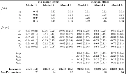
[image:24.612.149.487.107.431.2]Table 6. Sensitvity analysis: comparing different NMAR models (main parameters) : posterior estimates and standard deviations
No region effect Region effect
Model 1 Model 2 Model 3 Model 1 Model 2 Model 3
fZ(·)
p1 0.31 0.32 0.32 0.31 0.32 0.32
p2 0.23 0.25 0.24 0.23 0.25 0.24
p3 0.28 0.33 0.33 0.28 0.33 0.33
p4 0.12 0.15 0.16 0.12 0.15 0.16
fT|Z(·)
α0 9.95 (0.21) 10.06 (0.22) 10.07 (0.21) 9.82 (0.22) 9.83 (0.22) 9.86 (0.23)
α1 -0.84 (0.19) -0.84 (0.17) -0.85 (0.17) -0.88 (0.19) -0.84 (0.18) -0.86 (0.18)
α2 -0.85 (0.16) -0.94 (0.16) -0.96 (0.15) -0.81 (0.17) -0.86 (0.15) -0.87 (0.16)
α3 -0.84 (0.16) -0.69 (0.15) -0.65 (0.15) -0.84 (0.16) -0.75 (0.15) -0.73 (0.15)
α4 -0.54 (0.12) -0.62 (0.11) -0.62 (0.11) -0.60 (0.13) -0.69 (0.11) -0.70 (0.11)
1
σ2 0.66 (0.06) 0.65 (0.06) 0.65 (0.06) 0.67 (0.06) 0.68 (0.06) 0.68 (0.07)
b(s)1 – 0.51 (0.15) 0.71 (0.15) 0.73 (0.15)
b(s)2 – -0.10 (0.14) -0.03 (0.14) -0.03 (0.14)
b(s)3 – 0.18 (0.13) 0.22 (0.13) 0.22 (0.13)
b(s)4 – 0.25 (0.14) 0.26 (0.13) 0.26 (0.14)
Deviance 24580 (51) 23470 (77) 23240 (105) 24560 (53) 23420 (78) 23160 (113)
No.Parameters 20 24 32 24 28 36
Key
fZ(·) is modeled as in equation 12-15 using the conditional wise specification. pk fork= 1,· · ·,4
represent marginal probabilities for the four severe impairment variables in the order Lower Limb Function (ambulation); Upper Limb Function (manual); Intelligence Quotient; and Vision.
fT|Z(·) is modeled as in equation 7, with α0 is the intercept parameter; σ the scale parameter;
andα = (α1, . . . , α4), whereαk for k = 1,· · ·,4 are the covariate effect parameters for the four
severe impairment variables (order as above); For the survival model with additional variation due to region, b(s)j for j = 1,· · ·,4 represent fixed region effects (order: Scotland, the North of
England, Northern Ireland, Oxford, and Mersey as the baseline).
fR(r;ψ) is modelled by equations 17 and 18
Notes:
Model 1: Intercept only (MAR); Model 2: Intercept, covariate; Model 3: Intercept, covariate, time, censoring status.
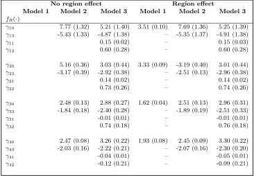
Table 7. Sensitvity analysis: comparing different NMAR models (NMAR parameters): poste-rior estimates and standard deviations
No region effect Region effect
Model 1 Model 2 Model 3 Model 1 Model 2 Model 3
fR(·)
γ10 7.77 (1.32) 5.21 (1.40) 3.51 (0.10) 7.69 (1.36) 5.25 (1.39)
γ13 -5.43 (1.33) -4.87 (1.38) – -5.35 (1.37) -4.91 (1.38)
γ11 0.15 (0.02) – 0.15 (0.03)
γ12 0.60 (0.28) – 0.60 (0.28)
γ20 5.16 (0.36) 3.03 (0.44) 3.33 (0.09) -3.19 (0.40) 3.01 (0.44) γ23 -3.17 (0.39) -2.92 (0.38) – -2.51 (0.13) -2.96 (0.38)
γ21 0.14 (0.02) – 0.14 (0.02)
γ22 0.73 (0.26) – 0.74 (0.26)
γ30 2.48 (0.13) 2.88 (0.27) 1.62 (0.04) 2.51 (0.13) 2.96 (0.31) γ33 -1.84 (0.18) -2.40 (0.28) – -1.89 (0.19) -2.51 (0.33)
γ31 -0.01 (0.01) – -0.01 (0.01)
γ32 0.74 (0.18) – 0.76 (0.18)
γ40 2.47 (0.08) 3.26 (0.22) 1.93 (0.08) 2.45 (0.09) 3.30 (0.22)
γ43 -2.03 (0.16) -2.22 (0.21) – -2.07 (0.16) -2.30 (0.20)
γ41 -0.04 (0.01) – -0.05 (0.01)
γ42 -0.12 (0.21) – -0.09 (0.21)
Key
fR(·) is modeled as in equation 17.
γ1 refers to the distribution of the missing data mechanism for the covariate lower limb
func-tion;
γ2refers to the distribution of the missing data mechanism for the covariate upper limb function;
γ3refers to the distribution of the missing data mechanism for the covariate cognitive function;
γ4refers to the distribution of the missing data mechanism for the covariate visual function;
The parameters γk0, γk1, γk2, γk3 for variable k (1...4) (above) represents and intercept value,
an effect due to the covariate, and effect due to the event time, and an effect due to the censoring status.
Notes:
Model 1: Intercept only (MAR); Model 2: Intercept, covariate; Model 3: Intercept, covariate, time, censoring status.
Figure 1. Kaplan-Meier estimates of survival for the severe and unknown impairments
LLF severe Age in years
Prop. alive
0 5 10 15 20 25
0.4
0.8
LLF missing Age in years
Prop. alive
0 5 10 15 20 25
0.4
0.8
ULF severe Age in years
Prop. alive
0 5 10 15 20 25
0.4
0.8
ULF missing Age in years
Prop. alive
0 5 10 15 20 25
0.4
0.8
IQ severe Age in years
Prop. alive
0 5 10 15 20 25
0.4
0.8
IQ missing Age in years
Prop. alive
0 5 10 15 20 25
0.4
0.8
Vision severe Age in years
Prop. alive
0 5 10 15 20 25
0.4
0.8
Vision missing Age in years
Prop. alive
0 5 10 15 20 25
0.4
0.8
Key