Time Variation in the Covariance between Stock
Returns and Consumption Growth
GREGORY R. DUFFEE∗
ABSTRACT
The conditional covariance between aggregate stock returns and aggregate consump-tion growth varies substantially over time. When stock market wealth is high relative to consumption, both the conditional covariance and correlation are high. This pattern is consistent with the “composition effect,” where agents’ consumption growth is more closely tied to stock returns when stock wealth is a larger share of total wealth. This variation can be used to test asset-pricing models in which the price of consumption risk varies. After accounting for variations in this price, the relation between expected excess stock returns and the conditional covariance is negative.
AFTER DECADES OF RESEARCH, financial economists have tentatively concluded that there are predictable variations in excess returns to the stock market. The uncertainty in this conclusion is partially driven by our inability to interpret comfortably these variations in a sensible model of asset pricing. In a world of rational investors who care about consumption, variations in expected excess returns should be driven by variations in either the amount of “consumption risk” in stock returns—the conditional covariance between stock returns and consumption—or the required compensation per unit of consumption risk. But attempts to link these potential explanations to the data have either failed empirically or have not been rigorously tested.
A major problem is that existing research has found little evidence for time variation in the conditional covariance between stock returns and aggregate consumption growth. Given this conclusion, there are only two interpretations we can place on time-varying expected excess returns in a consumption-based model. The first possibility is that investors are heterogeneous and there is time variation in the conditional covariance between stock returns and the consump-tion of marginal stockholders that is not matched by a similar variaconsump-tion at the aggregate level. The second possibility is the price of consumption risk varies through time. Neither possibility is easily tested empirically. Consumption data on individual investors is noisy and limited, while proxies for the price of con-sumption risk tend to be chosen based on the known behavior of expected stock returns, making the models close to tautological.
∗Haas School of Business, University of California at Berkeley. Thanks to the many seminar participants who have commented on earlier versions of this paper, and also to an anonymous referee, John Campbell, Karen Dynan, Kris Jacobs, Martin Lettau, and Sydney Ludvigson.
In this paper I re-examine the relation between aggregate stock returns and aggregate consumption growth. As econometricians we do not observe their conditional covariance, thus we attempt to infer it by projecting the product of innovations to stock returns and consumption growth on a set of instruments. Therefore, conclusions about the time variation in the conditional covariance hinge on the econometrician’s choice of instruments. I find that instruments related to the ratio of stock market wealth to consumption predict substantial time variation in the conditional covariance.
An important source of this predictive power is what I call the “composition effect,” which refers to the composition of total wealth. The role of the com-position effect in asset pricing was first noted by Santos and Veronesi (2003). Consumption moves with wealth. Wealth consists of both stock market wealth and non-stock-market wealth. At times when the share of stock market wealth in total wealth is relatively high, then (1) stock market wealth will be high rel-ative to total consumption and (2) the sensitivity of consumption to changes in stock market wealth will be relatively high. Hence, both the conditional covari-ance and the conditional correlation between stock returns and consumption growth will be above average when the ratio of stock market wealth to con-sumption is above average. This simple theory is strongly supported in U.S. data from 1959 to 2001. For example, point estimates of the conditional corre-lation between monthly stock returns and monthly consumption growth over this period range from roughly 0 to about 0.6, with the highest values reached at the tail end of the bull market that ended in 2000.
An unfortunate consequence of this evidence is that it increases the difficulty of explaining time variation in expected excess stock returns.1Existing research documents that expected excess returns tend to be high when stock valuations are relatively low, which is also when conditional covariances are relatively low. This pattern demands dramatically more time variation in the price of consumption risk to explain time variation in expected stock returns. We can think of the ratio of expected excess returns to the conditional covariance as the price per unit of consumption risk. When I take into account the lagged response of consumption to stock returns, I estimate that over the past 40 years this ratio has an interquartile range from 28 to 360. Therefore, in order to fit these data, a representative–agent model needs to imply that 10-fold swings in the price of consumption risk are common.
A more important consequence of this evidence is that it allows us to better test models that produce time variation in the price of consumption risk. Such models typically imply that there is some observable variable that can be used as a proxy for investors’ price of consumption risk. If the model is correct, the relation between conditional covariances and expected excess returns should depend on the level of this proxy. For example, when the price of risk is high, an increase in the conditional covariance should correspond to a larger increase in expected excess returns than when the price of risk is low. I test this hypothesis
1Santos and Veronesi (2003) arrive at a somewhat different conclusion, as I discuss at various
using various proxies for the price of consumption risk. The results are not encouraging. There is no statistically reliable evidence that, say, a higher level of surplus consumption (and therefore presumably a lower price of consumption risk) corresponds to a decreased sensitivity of expected excess stock returns to the conditional covariance.
The framework I use to produce these results is in the spirit of the instru-mental variables approach of Campbell (1987) and Harvey (1989). The product of ordinary least-squares innovations to stock returns and consumption growth is treated as an ex post covariance estimate. The projection of this product on a set of instruments is the estimated conditional covariance. This setup imposes little structure on the dynamics of the conditional covariance and is sufficiently f lexible to accommodate nonsynchronous dynamics between stock returns and consumption. I also verify the main results with a multivariate generalized autoregressive conditional heteroskedasticity (GARCH) model.
Section I presents the theoretical motivation behind the composition effect. Section II discusses the econometric approach and the data. Econometric de-tails are presented in Section III. Section IV documents time variation in the conditional covariance. Section V links this time variation to expected excess stock returns. Section VI uses a GARCH model to examine the conditional cor-relation. Concluding comments are offered in Section VII.
I. The Theoretical Motivation A. Consumption-Based Representative Agent Models
In consumption-based representative agent models, the stochastic discount factor is tied to the behavior of aggregate consumption. Therefore, conditional covariances between asset returns and aggregate consumption growth play a central role in determining expected excess returns. To fix ideas, denote the stochastic discount factor by exp(mt) and the log excess return to some asset fromt−1 totasrt. In this paper I focus on the excess return to the aggregate stock market. Ifmtandrtare jointly conditionally normally distributed, then no arbitrage implies
Et−1rt+ 1
2Vart−1(rt)= −Covt−1(rt,mt). (1) In equation (1) expectations are conditioned on information available at the end of periodt−1. The Jensen’s inequality term adjusts for the use of log returns over a discrete horizon.
Power utility, recursive utility, and habit formation models all expressmtas a function of aggregate consumption growth and perhaps other variables. For example, the habit formation model of Campbell and Cochrane (1999) implies
mt=k(st−1)−(1+λ(st−1))ct, (2) where st is a measure of surplus consumption andct is log-differenced per capita real consumption. Power utility is a special case in whichk(st−1)=logδ
(a constant) and 1+λ(st−1)=γ (also constant). A model such as Campbell and Cochrane’s habit formation implies
Et−1rt+ 1
2Vart−1(rt)=γt−1Covt−1(rt,ct) , (3) where γt is the state-dependent sensitivity of expected returns to the condi-tional covariance between consumption growth and stock returns. In other words, expected excess returns to the stock market equal the product of the price per unit of consumption risk and the amount of consumption risk in stocks. In Campbell and Cochrane,γt=1+λ(st).
An obvious way to test the time-series implications of (3) is to form conditional second moments (indicated with hats) and then estimate an equation such as
rt+ 1
2Vart−1(rt)=b0+bt−1Covt−1(rt,ct)+et, (4) wherebt−1is a parameterized observable proxy for the representative agent’s state-dependent price of consumption risk. Given the strong interest among academics and market professionals in identifying and explaining f luctuations over time in the expected aggregate stock returns, we might think that the literature would be rife with conditional tests such as (4). Yet they are almost nonexistent in published work. Attanasio (1991) and Ferson and Harvey (1993) study restricted versions of (4) whereb0=0 andbt−1is a constant. Yogo (2003) looks at the consumption of durables, while Li (2001) and Parker (2003) contain brief discussions of the variation in the conditional covariance. The main reason for this gap in the literature is that this research has identified only weak evidence of time variation in the conditional covariance.2 This is surprising because there is a compelling reason to believe that the conditional covariance varies through time.
B. The Composition Effect
Time variation in the conditional covariance arises naturally in any model in which the stock market does not account for all of investors’ wealth. A ma-jor source of this variation is variation in the conditional correlation between stock returns and consumption growth. As stock market wealth varies relative to the other determinants of aggregate consumption, so will the conditional correlation.
This point is first made clearly by Santos and Veronesi (2003) in an exami-nation of the relative importance of labor income to consumption. They build a model of risk-averse agents who invest in assets that pay stochastic dividends, where the stochastic processes followed by dividend growth are fairly general. Here I use a more simplistic model to illustrate the point. Investors consume dividends from their total wealth. Wealth consists of stock market wealth and
2There is stronger evidence if consumption data are not seasonally adjusted. See Attanasio
all other assets such as other claims on firms’ cash f lows (e.g., corporate bonds), real estate, and human capital. Group these other assets together and denote real dividends to stocks and all other assets asδs,tandδo,trespectively. Aggre-gate real consumption equals total dividends
Ct=δs,t+δo,t. (5) For tractability I assume that dividend growth rates for both the stock mar-ket and all other wealth are random walks with constant variances and equal growth rates g. This growth rate is a simple net rate, as are the other rates used in this model. Formally,
δs,t+1/δs,t=1+g+s,t+1, δo,t+1/δo,t=1+g+o,t+1. (6)
Again for tractability, I assume that investors are risk neutral and the real discount rate is rf. Risk neutrality is not important; it simply allows us to calculate easily the ex-dividend values of the stock market and all other wealth. These values are
Ws,t= 1+g rf −gδs,t , Wo,t= 1+g rf −gδo,t. (7) Therefore, the gross returns to these two forms of wealth are
Rk,t+1= Wk,t+1+δk,t+1 Wk,t+1 =1+rf + 1+rf 1+gk,t+1, k= {s,o}. (8)
The conditional variances of these returns are assumed to be constant over time. Denote them byσ2
s andσ2o, respectively. Denote their correlation byρ. Substitution of (7) into (5) allows us to write the change in consumption from
ttot+1 as Ct+1 Ct =φt Ws,t+1 Ws,t + (1−φt)Wo,t+1 Wo,t , (9)
whereφtis the share of stock market wealth in total wealth
φt≡ Ws,t
Ws,t+Wo,t.
(10) A similar derivation involving total wealth appears in Campbell (1996). Because his focus is on long-run behavior, he linearizes and replaces the time-varying coefficient φt with a constant coefficient. Lettau and Ludvigson (2001) and Jagannathan and Wang (1996) follow his lead. Here it is important to retain the time subscript inφtbecause the model implies that the conditional correla-tion between the return to the stock market and consumpcorrela-tion growth increases inφt. For example, the conditional correlation isρ whenφt=0 and is 1 when
With this model the conditional covariance between aggregate consumption growth and stock returns is
Covt Ct+1 Ct ,Rw,t+1 = 1+g 1+rf σ2 s φt+(1−φt) ρσo σs . (11)
This covariance depends onρσo/σs. The available evidence indicates that stock returns are highly volatile relative to the other determinants of consumption. (In the United States, the standard deviation of aggregate stock returns is about 15 times the standard deviation of consumption growth.) Therefore, this ratio is much less than 1, which implies that the conditional covariance is an increasing function ofφt. Asφtincreases, consumption growth becomes more volatile and more highly correlated with stock returns. Both effects raise the conditional covariance.
In practice, we do not observe the stock of nonfinancial wealth.3However, we can inferφtfrom the ratio of stock market wealth to consumption
φt= rf −g 1+g Ws,t Ct . (12)
Intuitively, when the ratio of stock market wealth to consumption is higher than usual, it is relatively more important in determining consumption.
Before we take this model to the data, we will have to make it a little more complicated. The complications are noted in Section II.B. Even with the compli-cations, a robust theoretical conclusion is that the composition effect induces a procyclical conditional covariance. Because stock prices are highly volatile and rise as the economy booms, stocks account for a larger share of total wealth in booms than in recessions. We know from the empirical literature on stock return forecastability that expected excess returns are countercyclical. Even without taking into account procyclical conditional covariances, researchers have strug-gled to understand the observed time variation in expected returns. Once time variation in covariances is introduced, the difficulty of explaining the behavior of expected returns is magnified substantially.
The conclusion that the composition effect complicates our ability to explain expected stock returns seems straightforward. However, Santos and Veronesi (2003) conclude that empirically, the composition effect actually helps to explain time variation in expected returns. They assume that there are two assets: human capital and stocks. Given this assumption, the ratio of human capital to consumption contains the same information as does the ratio of stock market wealth to consumption. We do not observe human capital, but we observe labor income, which is the dividend to human capital. Given certain restrictions on the dynamics of this dividend, the ratio of labor income to consumption will be negatively correlated with the conditional covariance between stock returns and consumption growth.
3In this simplistic model, we can calculate wealth if we observe dividends. But this relies on the
Santos and Veronesi use this logic to justify regressions of stock returns on the lagged ratio of labor income to consumption. They find a negative relation, consistent with their theory. (They do not consider the ratio of stock market wealth to consumption, nor do they check whether the ratio of labor income to consumption has predictive power for the conditional covariance.) I discuss the behavior of the labor income/consumption ratio in Section IV. Here it is sufficient to note that notwithstanding their results, the empirical analysis in this paper strongly supports the conclusion that conditional covariances and expected stock returns move in opposite directions over time.
C. The Composition Effect and Heterogeneous Agents
In a world of heterogeneous agents, an equation such as (4) can provide only indirect evidence on time variation in the risk-return tradeoff of stockhold-ers. Because stockholder consumption is more sensitive to stock returns than is nonstockholder consumption, the conditional covariance at the stockholder level will exceed the conditional covariance at the aggregate level. But the cen-tral issue here is whether time variation in the aggregate-level covariance is associated with time variation in the stockholder-level covariance.
To understand the relation between the aggregate-level and stockholder-level covariances, first note that with heterogeneous agents the composition effect works at both the aggregate level and at the stockholder level. In any rea-sonable model of the stock market and consumption, some part of aggregate consumption will be tied to stock market wealth. Therefore, the composition of the determinants of aggregate consumption will vary over time with the level of the stock market. When the aggregate value of stocks is high relative to other determinants of consumption, a larger share of aggregate consumption is sensitive to stock market wealth. The result is a relatively high conditional covariance between aggregate consumption and aggregate stock returns, just as in the representative–agent setting.
At the stockholder level, the magnitude of the composition effect depends on the stockholder’s stock wealth as a fraction of her total wealth. The relation is not monotonic. To simplify this discussion, assume that stock returns are uncorrelated with returns to non-stock wealth. Then the counterpart of (11) for agentisimplifies to Covt Ci,t+1 Cit ,Rw,t+1 = 1+g 1+rfσ 2 sφit, (13)
where φit is the ratio of stock market wealth to total wealth for agent i. The variability of the conditional covariance for agentidepends on the variability of
φit, which in turn depends on the level ofφit. Consider, for example, the effect on
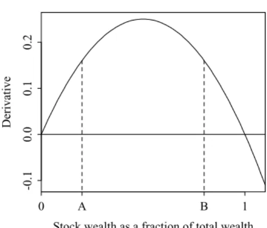
φitof an increase in the value of the aggregate stock market. If agentieither has no wealth in stocks or has her entire wealth invested in the stock market, there is no effect onφit and the conditional covariance is constant. More generally, the derivative ofφitwith respect to the log of investori’s stock market wealth isφit(1−φit), which is plotted in Figure 1.
Stock wealth as a fraction of total wealth Derivative 0 A B 1 -0.1 0.0 0.1 0.2
Figure 1. Derivative of (stock wealth/total wealth) with respect to log stock wealth.Total wealth is the sum of stock market wealth and non-stock wealth. The fraction held in the form of stock market wealth isφ. This figure plots the derivative ofφwith respect to log stock market wealth, which is equivalent to the sensitivity ofφto the return to the stock market. The amount of non-stock wealth is held constant in computing this derivative.
What is a reasonable value ofφit for a typical stockholder? As discussed in Jagannathan and Wang (1996), the contribution of the stock market to aggre-gate consumption is fairly low. (For example, aggreaggre-gate dividends were less than 3% of total income from 1959 through 1992.) Thus, for a representative agent, the typical fraction of wealth in stocks is on the left side of the figure, say at point “A.” With heterogeneous agents, stock holdings are concentrated among investors who hold a larger fraction of their wealth in stocks than does the typical consumer. If that fraction lies between “A” and “B” in the figure, then the sensitivity ofφitto the stock market is higher for stockholders than it is for the aggregate economy.
This argument suggests that variation in the marginal investor’s conditional covariance is a scaled-up version of variation in the aggregate conditional co-variance. If so, estimating an aggregate-level equation such as (4) helps to evaluate heterogeneous-agent models as well as representative-agent models. More concrete conclusions must rely on specific heterogeneous-agent models. Unfortunately, the theory of asset markets with heterogeneous agents is not as well developed as is the corresponding theory with representative agents. In particular, the behavior of conditional correlations is hard to study because dynamic equilibrium models such as Basak and Cuoco (1998) and Chan and Kogan (2002) have a single random variable. (Shapiro (2002) is a notable ex-ception.) We cannot even be sure that the sensitivity of the marginal investor’s φitto the value of the stock market is positive. In the model of Basak and Cuoco, stockholders have a leveraged position in stocks. (In Figure 1 this corresponds to a point to the right of “1” on thexaxis.) An implication of their model is that stockholders’ conditional covariance is countercyclical because an increase in the stock market lowers stockholders’ leverage and hence lowers the volatil-ity of their consumption. Thus, in the absence of either a formal model of the
composition effect in a world of heterogeneous agents or detailed information about the wealth of the marginal stockholder, any conclusions drawn from an equation such as (4) about the validity of heterogeneous-agent models should be tempered with caution.
II. The Econometric Approach A. The Regressions
Period-texcess stock returns and consumption growth can be written as sums of one-step-ahead expectations and innovations
rt=Et−1rt+rt, ct=Et−1ct+ct. (14) The product of the innovations, when projected on investors’ information set at timet−1, is the conditional covariance.
As econometricians, we do not observe either the true innovations or the en-tire set of conditioning information available to investors. A standard approach, which I follow here, is to use forecasting regressions to construct fitted residuals as proxies for true innovations. The product of the fitted residuals is then pro-jected on a set of instruments identified by the econometrician. The forecasting regressions for returns and consumption growth can be written as
rt =arYr,t−1+er,t−1,t−1,t, (15)
ct=acYc,t−1+ec,t−1,t−1,t, (16)
wherearandacare parameter vectors and the vectorsYr,tandYc,tare realized in periodt or earlier. I refer to these regressions as “zero-stage” regressions, to distinguish them from the usual first-stage and second-stage instrumental variable regressions that are introduced below. The first time subscript on the residuals refers to the date of the instrument vector (i.e., the period at which the forecast is made). The second and third time subscripts are the starting and ending dates of the dependent variable. Here those subscripts aret−1 andt; the stock return is calculated from the end of periodt−1 to the end of periodt, and consumption growth is the log change in consumption fromt−1 tot. Not all of these subscripts are necessary to uniquely denote residuals of (15) and (16), but they will be useful later when we considern-period-ahead forecasts of longer horizon stock returns and consumption growth.
Denote the product of the fitted residuals as
Cov∗(rt,ct)≡eˆr,t−1,t−1,teˆc,t−1,t−1,t. (17) The asterisk indicates an ex post estimate. The ex post estimate is projected on a set of instrumentsZt−1to produce a conditional covariance estimate:
Cov∗(rt,ct)=avZt−1+µt, (18)
Equation (18) is the first-stage regression. I estimate it with OLS and test hy-potheses aboutavwith Wald statistics. I use a robust estimate of the variance– covariance matrix, which implies that the statistics have asymptoticχ2 distri-butions.
The following second-stage regression is estimated with instrumental vari-ables: rt+ 1 2Var ∗(rt)=b 0+[b1+b2pt−1]Cov∗(rt,ct)+wt. (20) This regression is in the spirit of the instrumental regressions in Campbell (1987) and Harvey (1989). The second term on the left side is an ex post estimate of the variance of stock returns,
Var∗(rt)≡eˆr2,t−1,t−1,t. (21) The term in square brackets on the right-hand side of (20) is an observable proxy for the conditional price of consumption risk, which I also refer to asbt:
bt ≡b1+b2pt−1. (22) The base case of bt is power utility, or b2=0. A more general case is where the observable variableptpicks up time variation in investors’ willingness to bear consumption risk. For example, Campbell and Cochrane’s model could be tested using bt =b1+b2sˆt−1, where ˆst−1 is a proxy for surplus consumption. The constant termb0 forces identification of the relation betweenpt and the price of risk to be picked up exclusively through a nonlinear relation between the conditional covariance and expected excess stock returns.
I use the generalized method of moments (GMM) technique of Hansen (1982) to estimate jointly the zero-stage regressions and second-stage instrumental variable regression. This allows the standard errors of the second-stage regres-sion to incorporate the uncertainty in the fitted residuals owing to parameter uncertainty in the zero-stage regressions. In Section III.A, I evaluate the finite-sample properties of this method using Monte Carlo simulations.
B. Data Description and the Choice of Instruments
I use monthly data. Monthly consumption is measured by Bureau of Eco-nomic Analysis estimates of monthly per capita expenditures on nondurables and services, which are available beginning in January 1959. Expenditures are in 1996 dollars. Monthly consumption growth is defined as log-differenced consumption. I measure excess monthly returns to the aggregate stock market by the log return to the CRSP value-weighted NYSE/Amex/Nasdaq index less the continuously compounded yield on a 1-month Treasury bill as of the end of the previous month. The last observation of stock returns in my sample is December 2001.
The choice of instruments included in the vectorZt used in the first-stage and second-stage regressions is motivated by the composition effect. The first
Date ME/C 1960 1970 1980 1990 2000 1.0 2.0 3.0
A. Stock market wealth/consumption
Date
CAY
1960 1970 1980 1990 2000
-0.04
0.0
B. Detrended consumption-wealth ratio
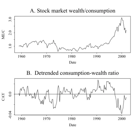
Figure 2. Ratios of wealth to consumption.The top panel plots the ratio of the market capi-talization of publicly traded stocks to total consumption on nondurables and services. The bottom panel plots the detrended consumption–wealth ratio introduced in Lettau and Ludvigson (2001).
instrument is the ratio of stock market wealth to consumption. Stock mar-ket wealth is measured by the month-end marmar-ket capitalization of the CRSP value-weighted index, expressed in real per capita terms for comparability to the consumption data. I denote this ratio by ME/C. Recall that one of the sim-plifying assumptions in the model of Section I.B is that the variance of stock returns is constant. However, stock return volatility temporarily falls (rises) after the market rises (falls).4This means that an increase in ME/C is accom-panied by a short-run decline in stock return volatility. This damps the role of the composition effect; the decline in volatility tends to lower the conditional covariance. To control for this effect, I also include lagged excess stock returns in the instrument vector. Denoting the sum2i=0rt−i byRETqt, I includeRET
q t andRETqt−3inZt.
Not surprisingly, the ratio ME/C is related to the consumption–wealth ra-tio cay introduced by Lettau and Ludvigson (2001). Their ratio is the trend deviation in the log consumption–wealth ratio, where wealth includes capital-ized labor income. The two ratios are plotted in Figure 2. It is apparent from
4This pattern was discovered by Black (1976) and is the subject of a large literature. See, for
the figure that, although the two ratios move inversely (their correlation is about−0.58), ME/C is much more persistent than iscay. In quarterly data the first-order autocorrelation coefficient of ME/C is 0.96, compared with 0.85 for
cay. Therefore,cay is more closely related to the business cycle, as noted by Lettau and Ludvigson. The ratio ME/C is picking up lower frequency variation in the relative importance of the public stock market. Part of the low-frequency variation in ME/C may be variation in the proportion of stocks that are traded publicly versus privately. Small, less-well-known firms are probably better able to access capital through issuance of publicly traded stock today than they were in the 1960s.
The relevant ratio from the perspective of the composition effect is ME/C. Nonetheless,caylikely contains independent information about the conditional covariance, both because of the business cycle link and because it forecasts stock return volatility, as documented by Lettau and Ludvigson (2002a). (I look at predictions of stock return volatility in Section VI.) I therefore also include
cayin the instrument vector.5Since the consumption–wealth ratio is defined using quarter-end data, I assume that the observation available at the end of the first two months in each quarter is the value as of the end of the previous quarter.
Many variables in macroeconomics and finance exhibit persistent f luctua-tions in volatility. This empirical regularity suggests that lags of ex post co-variance estimates should be included inZt. From an econometric perspective, it is more useful to use a slightly different proxy for the ex post covariance: the product of demeaned stock returns and demeaned consumption growth. The time series properties of this product are close to those of the ex post co-variance, but unlike the ex post covariance this product does not depend on parameter estimates from the zero-stage regressions. To limit the number of explanatory variables, I use 3-month sums instead of the individual monthly products. These sums are denoted by
CVt= 2
i=0
(ct−i−c)(rt−i−r¯). (23) I include four nonoverlapping lags of CVt inZt. For completeness the set of instruments is reported in the following equation:
Zt =
1, (ME/C)t,RETqt,RET q
t−3,cayt,CVt,CVt−3,CVt−6,CVt−9 . (24) I do not include the ratio of labor income to consumption in this set of instru-ments because any information in this ratio should be subsumed in the ratio of stock market wealth to consumption. Nevertheless, to compare my results to those of Santos and Veronesi (2003), I report some results in which I use the ratio of labor income to consumption instead of the ratio of stock market wealth
5The forecasting power ofcayfor stock returns is somewhat controversial. The look-ahead bias
of the cointegrating relation is the subject of Brennan and Xia (2002), while Hahn and Lee (2001) argue the forecasting power is not stable. See also Lettau and Ludvigson (2002b).
to consumption. I compute this ratio using quarterly data following the defi-nition of labor income in Lettau and Ludvigson (2001). As withcay, I assume that the value available at the end of the first 2 months in each quarter is the value as of the end of the previous quarter.
Two other instrument vectors are used in this paper. They areYc,t, used to construct fitted consumption growth residuals, andYr,t, used to construct fitted stock return residuals. Monthly consumption growth is autocorrelated, thus I include inYc,ta constant term and monthly consumption growth for monthst through t−2. I experimented with a larger set of instruments that included stock returns. These experiments led to the conclusion that the results in this paper are unaffected by the precise composition ofYc,t. The vectorYr,tconsists of a constant and the consumption–wealth ratiocay. I experimented with also including the dividend/price ratio and the slope of the term structure. The use of this larger information set has only a minimal effect on the results, thus I use the smaller set here.
Higher frequency data allow us to produce more accurate estimates of sec-ond moments (see, e.g., Andersen et al. (2003)). I use the highest frequency consumption data available. Stock return data are available at higher frequen-cies, thus I could produce more accurate estimates of the ex post variance of stock returns to use as the Jensen’s inequality adjustment on the left-hand side of (20). In practice, nothing is gained by improving the accuracy of this variance estimate because it contributes little to the overall variation of the left-hand side of the equation. The standard deviation of the log excess return is around 25 to 30 times the standard deviation of the Jensen’s inequality term, regardless of how the variance is estimated. The ratio of standard deviations of 1-month-ahead forecasts of these components is similar. (These results are not shown in any table.) Therefore, I do not use higher frequency stock return data in this paper.
C. Specifications of the Price of Consumption Risk
I consider various specifications of the price of consumption risk bt=b1+
b2pt−1. The first is power utility, orb2=0. Withb2=0, I consider three choices ofpt−1. They are a measure of surplus consumption, the consumption–wealth ratio, and the dividend–price ratio. The motivation for surplus consumption is the implication of some habit formation models that the price of consump-tion risk should vary with the level of current consumpconsump-tion relative to past consumption. Wachter (2002) proposes a measure of past consumption growth that arises naturally in habit formation models. I follow her suggestion and define a proxy for surplus consumption at the quarterly frequency as
ˆ st= 1− 1−40 39 j=0 jc(t−j), (25)
with the decay factor=0.96. For consistency with Wachter, the notation in this equation differs from that used elsewhere in this paper. In (25), time is
measured in quarters andctrefers to the log change in real per capita quar-terly consumption on nondurables and services. My proxy for surplus consump-tion at the monthly frequency is the most recent quarterly measure of surplus consumption.
The use of the consumption–wealth and dividend–price ratios is motivated by the possibility that the price of consumption risk may vary over time for reasons unrelated to habit. Such variations are likely to show up incayor D/P. A change in risk tolerance will alter the level of expected returns required by investors. Holding constant the time path of future cash f lows, this change in expected returns will change stock valuations relative to dividends and to the long-run cointegrating relation among stock market wealth, consumption, and labor income, as discussed by Campbell and Shiller (1988) and Lettau and Ludvigson (2001). I denote the dividend price ratio at the end of the montht
as (D/P)t, where the numerator is the sum of dividends paid in the previous 12 months.
III. Details
In this section I discuss three issues. First, I report Monte Carlo evidence on the properties of the estimation procedure described in the previous sec-tion. Second, I consider how to choose the horizon over which consumption growth should be measured. The natural lumpiness of consumption expendi-tures, combined with the method used to measure such expendiexpendi-tures, implies that the “contemporaneous” relation between stock returns and consumption growth may appear as a relation between time-t stock returns and time-(t+τ) consumption growth. Third, I describe how I estimate the relation be-tween expected stock returns and conditional covariances when both stock returns and consumption growth are measured over horizons longer than a month. This section is unavoidably tedious. For those readers who are unin-terested in the details, the next two paragraphs summarize the results of this section.
The Monte Carlo evidence indicates that standard GMM statistical tests for the presence of time variation in the conditional covariance (the first-stage regression) are well behaved. Statistical GMM tests of the null hypothesis that the conditional covariance has no predictive power for returns (the second-stage regression) are reasonably well behaved (e.g., true critical values for relevant
t-statistics are within 10–15% of asymptotic critical values) as long as there is a modest amount of true variation in the conditional covariance. Alternative estimation procedures, such as limited information maximum likelihood, do not have better finite-sample properties.
To address the slow adjustment of consumption, I use two measures of the covariance between stock returns and consumption growth. The first, which ignores slow adjustment, is the covariance between montht’s stock return and consumption growth from montht−1 to montht. The other is the covariance between montht’s stock return and consumption growth from montht−1 to month t +3. I conclude that given the hypotheses of interest in this paper, there is no obvious reason to prefer one of these measures. Finally, I use sums
of monthly ex post covariance estimates as ex post estimates of covariances over horizons longer than a month.
A. Monte Carlo Evidence
I use Monte Carlo simulations to investigate the properties of the economet-ric methodology. There are two reasons why the usual GMM asymptotics may be inappropriate here. First, the instruments used to construct conditional co-variances are weak. Second, there is an errors-in-variables problem created by the fact that we do not observe true residuals.
The properties of the instrumental variables regression (20) depend on the information in the instruments. Staiger and Stock (1997) suggest the instru-ments should be treated as weak if theF-statistic in the first-stage regression is small; say, less than 10. Kleibergen (2002) develops an instrumental variables statistical test that is robust to the presence of weak instruments. He uses limited information maximum likelihood (LIML) to estimate the second-stage regression and tests hypotheses using hisK-statistic. The advantage of LIML and Kleibergen’s test is that they are robust to weak instruments.
The econometric setting in this paper is more complicated than that studied in Kleibergen because here there are “zero-stage” regressions used to construct the residuals to stock returns and consumption growth. Unfortunately, the analysis of more general GMM estimation in the presence of weak instruments is in its infancy.6Stock, Wright, and Yogo (2002) suggest implementing GMM using the continuous-updating estimator of Hansen, Heaton, and Yaron (1996).
The errors-in-variables problem can be seen by expanding the product of fitted residuals into true residuals and errors in conditional expectations
Cov∗(rt,ct)=[rt+(Et−1rt−aˆrYr,t−1)][ct+(Et−1ct−aˆcYc,t−1)]. (26) Take the expectation of both sides with respect to the instrument vectorZt−1
ECov∗(rt,ct)Zt−1
=E(rtct|Zt−1)+ E[(Et−1rt−aˆrYr,t−1)(Et−1ct−aˆcYc,t−1)|Zt−1]. (27) If both the OLS forecasts of returns and the OLS forecasts of consumption growth differ from investors’ forecasts, then the second term on the right-hand side of (27) contaminates the proxy for the conditional expectation ofrtct. This errors-in-variables problem is basically the same as that identified by Pagan and Ullah (1988) in their discussion of regressions of stock returns on estimates of conditional variances. This problem has no effect under the null hypothesis that the price of consumption risk is zero. However, if this price differs from zero, the errors-in-variables problem results in inconsistent estimates of the parameters in (20).7
6Stock and Wright (2000) discuss asymptotic distribution theory for GMM estimators in this
case.
7One way to circumvent this problem is to explicitly treat the conditional covariance as a latent
To implement the Monte Carlo simulations, I model the evolution of the rel-evant variables with a vector autoregression (VAR). The variables in the VAR are (demeaned) monthly excess stock returns, log consumption growth, the de-trended consumption–wealth ratio, and the ratio of stock market wealth to consumption growth. (The ratio ME/C cannot be recovered from the combina-tion of stock returns and consumpcombina-tion growth because of f lows in and out of the stock market.) I do not impose any cointegrating relations among the variables. Shocks are drawn from a multivariate normal distribution. Because I construct residuals to consumption growth with a third-order autoregression (AR(3)), I also include two lags of consumption growth in the VAR. Stack these variables in a vectorxtwhere the first two variables are stock returns and consumption growth and the final two variables are lags 2 and 3 of consumption growth. Then the VAR is
xt= Axt−1+µt, Et−1(µt)=0, Et−1(µtµt)= t 0(2×2) 0(2×4) 0(2×2) . (28)
I set the first four rows of the parameter matrix A to the parameters from OLS estimation of the VAR over the sample period examined in this paper. (Exceptions to this are noted below.) The remaining two rows are determined by the companion form. I use two versions oft. One is a constant, set equal to the sample variance–covariance matrix of the residuals from OLS estimation of the VAR. The other version is identical except for the covariance between innovations in stock returns and consumption growth. I assume the conditional covariance varies over time because the conditional correlation changes over time. The setup is
12t=
(11)(22)ρt, (29)
where
ρt=ρ¯+α(ME/C)t−1. (30)
I setαto 0.35. This choice generates variability in the conditional covariance similar to that observed in the sample. The mean ¯ρ is set to the corresponding sample correlation. The conditional correlationρtmust be bounded in order to ensure the invertibility oft. If the above equation results in a correlation less than−0.36 or greater than 0.56,ρtis set to the relevant bound.
I produce three sets of Monte Carlo simulations that differ in the dynamics of returns and/or covariances. All of them satisfy the null hypothesis that the conditional covariance has no true forecast power for stock returns:
1. Neither conditional expectations of stock returns nor conditional covari-ances vary over time. For this hypothesis, I replace the first row of theA
matrix with zeros.
2. Conditional expectations of stock returns are constant and conditional covariances vary over time. Here the first row ofAis also zero, and covari-ances are produced with (29) and (30).
3. Conditional expectations of stock returns vary over time, and conditional covariances are constant. Here the first row of A is given by the OLS sample estimates.
A single simulation proceeds as follows. A panel of 515 monthly observations is generated with the specified process. (This is the length of the actual data sample.) Given this simulated data, I estimate the zero-stage regressions and use the results to construct ex post estimates of the covariance between stock returns and consumption growth. I then estimate the first-stage and second-stage regressions (18) and (20). In the latter regression, I set the parameterb2 to 0.
I estimate the second-stage regression with both asymptotically efficient GMM (jointly with the zero-stage regressions) and LIML, following Kleiber-gen’s methodology. The weighting matrix for GMM estimation is calculated using residuals from the OLS estimation of both the zero-stage and second-stage regressions. Experiments with the continuous-updating GMM estimator of Hansen et al. (1996) revealed that in this setting it has worse properties than LIML. Thus I do not discuss the results for this alternative estimator.
Table I summarizes the results of the first-stage regressions and GMM esti-mation of the second-stage regressions. The results for the first-stage regression are straightforward. The test of the hypothesis that the conditional covariance is predictable has reasonable size properties under the null of no predictabil-ity. The relevant results are in rows 1 and 3 of the table. Differences between
Table I
Finite-Sample Properties of the Estimation Procedure
This table summarizes the empirical distribution of asymptoticp-values and test statistics calcu-lated from 1,000 Monte Carlo simulations. A vector autoregression is used to simulate 515 monthly observations of excess stock returns, consumption growth, the ratio of stock market wealth to total consumption ME/C, and the consumption–wealth ratiocay. Given a simulated dataset, innovations to stock returns and consumption growth are constructed with OLS (zero-stage regressions). The prod-uct of these innovations is an ex post covariance estimate. In the first-stage regression, the ex post covariance estimate is regressed on a set of instruments. In the second-stage regression, excess stock returns are regressed on the ex post covariance estimate using the same set of instruments. The second-stage regression is estimated using asymptotically efficient GMM (incorporating the zero-stage regressions).
First Stage Regression Second Stage Regression
Freq. thatχ2-Stat Empirical Critical
>Asymp.p-Value Values for thet-Statistic
Mean Mean Median
Null F-Stat 10% 5% t-Stat t-Stat 0.025 0.05 0.95 0.975
Constant mean return, 1.00 0.127 0.058 0.00 −0.03 −1.87 −1.61 1.62 1.75 constant covariance
Constant mean return, 2.65 0.754 0.672 −0.33 −0.37 −2.16 −1.91 1.35 1.64 stochastic covariance
Stochastic mean return, 1.00 0.117 0.059 0.03 0.12 −2.45 −2.26 2.33 2.55 constant covariance
the empirical and asymptotic values are not large. For example, if neither re-turns nor conditional covariances are forecastable, the null is rejected in less than 6% of the simulations when the 5% critical value is used. The power of the first-stage regression under the alternative hypothesis (29) is reasonably high for the chosen value ofα. The relevant results are in the second row. The null hypothesis is rejected about 70% of the time at the 5% significance level. The typicalF-statistic is about 2.6, which is close to the empiricalF-statistics reported in Section IV.
The results for the second-stage regression depend on the specification of the null. First examine the case of unpredictable stock returns and predictable co-variances. These results are in the second row of the table. I report summary information aboutt-statistics of the estimates ofb1in (20) rather than informa-tion about the estimates themselves because the distribuinforma-tion of thet-statistics is more robust to variations in the process for generating conditional covari-ances.8When covariances are predictable and returns are not, thet-statistics are negatively biased. The explanation for the bias is consistent with the logic of Stambaugh (1999). If the value of ME/C at monthtis higher than its sample mean, then stock returns prior totare likely higher than their sample mean, and stock returns aftertare thus likely lower than their sample mean. This in-duces a spurious negative relation between ME/C at monthtand future stock returns. Since the conditional covariance is positively associated with ME/C, there is also a spurious negative relation between the conditional covariance and future stock returns. Therefore, to reject at the 5% level the null of no pre-dictability in returns in favor of the hypothesis that the conditional covariance predicts returns, thet-statistic onb1must be less than−2.16 or greater than 1.64.
The magnitude of this bias is, of course, lower when the true relation be-tween ME/C and the conditional covariance is weaker. At the extreme of no relation (the first row in the table), the bias disappears and the standard criti-cal values for the second stage regression are excessively conservative for both positive and negative parameter estimates. These results lead to a somewhat counterintuitive conclusion: when we are more confident about the presence of predictability in the conditional covariance, we must use more stringent critical values in the second-stage regression.
Given the existing research documenting predictability in stock returns, per-haps the most relevant case is when returns are predictable and conditional covariances are constant. To reject this null, we should rely on the first-stage regression. The third row of the table reports that the true critical values for the second-stage regression are much larger (in absolute value) than standard critical values. The problem in this case is that because we are using the same variables that predict returns to predict the conditional covariance, any spuri-ous predictive power for the conditional covariance will necessarily show up as predictive power for expected returns as well.
8This conclusion is based on experimentation with alternative processes for the conditional
The table does not report the results of LIML estimation because the Monte Carlo results indicate that LIML offers no advantages to GMM. The finite-sample properties of theK-statistic are substantially different from the corre-sponding asymptotic properties. The statistic is a measure of the distance of the parameter estimate from zero and has an asymptoticχ2distribution. Like the GMM estimate, the LIML estimate is biased. Under the null of constant mean returns and stochastic covariances, the empirical 5% critical value for the
K-statistic is 5.25 conditional on a negative LIML estimate. Conditional on a positive LIML estimate, this critical value is only 3.15. (The asymptotic critical value is 3.84 and does not depend on the sign of the estimate.) Viewing the same issue from a slightly different perspective, 9.2% of the negative estimates ofb1haveχ2values that exceeded the asymptotic 5% critical value.
There are three messages to take from these simulations. First, if the first-stage regression does not provide strong statistical evidence of time-varying conditional covariances, then we do not know what critical values to use in the second-stage regression. Second, if we can confidently reject the null of constant conditional covariances, the magnitude of this variation does not need to be large in order to produce reasonable results from the second-stage regression. AnF-statistic of about 2.5, although weak in the Staiger/Stock sense, appears sufficient. Third, there is no standard estimation procedure that dominates GMM.
B. The Horizon Used to Measure Consumption Growth
A well-known empirical result is that a period-tstock return shock is posi-tively correlated with measured aggregate consumption growth in both period
tand future periods. Grossman, Melino, and Shiller (1987) show that a positive correlation between period-treturns and period-(t+1) aggregate consumption growth is created by the time averaging that is built into measured consump-tion.9Lynch (1996) and Gabaix and Laibson (2001) note that transactions costs that delay adjustments to consumption can produce nonzero correlations over longer intervals. Thus the purely contemporaneous covariance between returns and consumption growth underestimates the true covariance. For example, a power utility model written in terms of measured aggregate consumption in-stead of the instantaneous consumption of a consumer that faces no transaction costs implies (see Gabaix and Laibson (2001))
Et−1rt+ 1
2Vart−1(rt)=γCovt−1(rt,ct+K∗−ct−1) , (31) whereK∗ is sufficiently large. This intuition suggests that we should replace the OLS forecasting regression for consumption growth (16) with a multiperiod counterpart
ct+k−ct−1=acYc,t−1+ec,t−1,t−1,t+k. (32)
The form of regression (20) is unchanged except for the replacement of the single-period fitted residual ˆec,t−1,t−1,t with the multiperiod residual ˆ
ec,t−1,t−1,t+k. Denote the corresponding ex post covariance by
Cov∗(rt,ct+k−ct−1)≡eˆr,t−1,t−1,tˆec,t−1,t−1,t+k. (33) Then the instrumental variables regression is
rt+ 1 2Var
∗(r
t)=b0+[b1+b2pt−1]Cov∗(rt,ct+k−ct−1)+wt. (34) We can setk=0 in (32) and (34) to recover the regressions (16) and (20).
Notwithstanding the logic underlying (31), for the purposes of this paper it is not clear that an empirical implementation that usesk>0 is superior to an implementation that usesk=0. Gabaix and Laibson emphasize the effect of
kon the ratio of mean excess returns to the unconditional covariance between stock returns and consumption growth. In (34) these unconditional moments are effectively picked up byb0, which is not of direct interest. Under the null hypothesis that the price of consumption risk is zero, the choice ofk has no effect. Under an alternative hypothesis the critical issue is how the choice ofk
affects the power of the statistical test.
To understand the effect of k on the power of the test, first note that the left-hand side of (32) is the sum ofksingle-period changes in log consumption. Therefore, we can write the multiperiod residual as the sum ofksingle-period residuals. These are the residuals from forecasts made att−1 ofct,ct+1, and so on. Similarly, we can write the product of the fitted residuals to stock returns and multiperiod consumption growth as the sum ofkproducts of fitted residuals to stock returns and single-period consumption growth:
Cov∗(rt,ct+k−ct−1)= k j=0 ˆ er,t−1,t−1,teˆc,t−1,t−1+j,t+j. (35)
Each of the ex post covariance estimates on the right-hand side of (35) is the sum of its conditional expectation and a residual:
ˆ
er,t−1,t−1,teˆc,t−1,t−1+j,t+j =Cov(rt,ct+j|Zt−1)+nt−1,t−1+j,j. (36) The first subscript on the noise term refers to the date of the instrument vectors used to construct the fitted residuals. The second and third are the beginning and ending dates used to define the change in log consumption. We can think of these ex post covariances as the sum of a signal (the conditional covariance) and noise (nt−1,t−1+j,j). Increasing k, or in other words, adding additional ex post covariance estimates to (35), increases both the total signal and the total noise. From the perspective of hypothesis testing, the net effect depends on the change in the total signal to total noise.
An example makes this clear. Assume the true model is power utility plus transaction costs, so that expected excess returns are proportional to the con-ditional covariance between returns and consumption growth overK∗ periods.
Also assume that investors and econometricians are working with the same information set, so we can ignore any errors-in-variables problem. Denote the conditional covariance between returns and long-horizon consumption growth asBt−1:
Cov(rt,ct+K∗−ct−1|Zt−1)≡Bt−1. (37) Then excess returns are the sum of a term proportional toBt−1plus a residual
rt+ 1
2Var(rt|Zt−1)=γBt−1+r,t. (38) To simplify the analysis, assume that for k≤K∗, the conditional covariance between returns and thej-period-ahead consumption growth is proportional to
Bt−1: Covt−1(rt,ct+j)=ρjBt−1, ρj ≥0, K∗ j=0 ρj =1. (39)
In other words, these conditional covariances all move together. We can combine this equation with (38) to show that for arbitraryk,
rt+ 1 2eˆ 2 r,t−1,t−1,t = γ k j=0 ρj Cov∗(rt,ct+k−ct−1) + r,t− γ k j=0 ρj k j=0 nt−1,t−1+j,t+j + 1 2 ˆ er2,t−1,t−1,t−Var(rt|Zt−1) . (40)
The term in square brackets is unforecastable with the instrumentsZt−1. Now consider the instrumental variables regression (34) withb2=0. The de-pendent variable in the regression is the left-hand side of (40). The explanatory variable is the ex post covariance on the right-hand side of (40). Therefore, the estimate ofb1should approach the coefficient in front of the ex post covariance. More precisely, for a givenk, the instrumental variable estimate ofb1, denoted
ˆ b1{k}, satisfies plim ˆb1{k}= γ k j=0 ρj . (41)
Fork<K∗, this plim exceeds the true coefficient of relative risk aversion, a re-sult consistent with the intuition of Gabaix and Laibson. Therefore, an increase
inktends to push the parameter estimate toward the true value ofγ. However, the asymptotic t-statistic of ˆb1{k} does not necessarily increase with k. If we ignore the dependence of ˆer,t−1,t−1,teˆc,t−1,t−1,t+k on first-stage parameter esti-mates, it is straightforward to show that the asymptotict-statistic is inversely proportional to the standard deviation of the term in square brackets in (40). Therefore, from the perspective of the power of the test that b1=0, adding an additional lead of consumption growth has two offsetting effects. The first is that an additional noise term is added to the sumkj=0nt−1,t−1+j,t+j. The second is thatkj=1ρj increases, which dampens the effect of the sum of noise terms.
It is hard to say more about the effects of k without assuming something about the joint distribution of the error termsrt,nt−1,t−1+j,t+j and ˆer2,t−1,t−1,t− Var(rt|Zt−1)). If they are jointly uncorrelated, the effect ofk depends on the ratio k j=0 Var(nt−1,t−1+j,t+j) k j=0 ρj . (42)
A higher value ofkresults in a less powerful test if it increases this ratio. The extreme case is if excess stock returnsrtand future consumption growthct+j are uncorrelated. Then their product is pure noise, so including thejth lead of consumption results in lower power.
In summary, the choice ofkhas no effect under the null and has an ambiguous effect on power under alternative hypotheses. The best choice ofklikely depends on the precise alternative hypothesis of interest. I adopt an ad hoc procedure for choosingk based on the unconditional sample covariances between fitted residuals to stock returns and leads of consumption growth.
Table II reports the unconditional covariance between innovations in stock returns and consumption growth, where the innovations are residuals from the first-stage regressions (15) and (16). The sample period is February 1960 through December 2001. The relation between stock returns and consumption growth is the strongest for contemporaneous consumption growth. The covari-ances drop off to zero beyondj=3. I therefore, focus on two different measures of ‘contemporaneous’ consumption growth. They are the growth in consumption fromt−1 tot(k=0) and fromt−1 tot+3 (k=3), respectively.
C. The Stock Return Horizon
Most of the data used in this paper are available at a monthly frequency, which leads me to focus on the predictability of monthly returns. For compa-rability with other research, I also predict returns over longer horizons using conditional covariances appropriate for those horizons.
Table II
The Relation between Aggregate Stock Returns and Real Consumption Growth
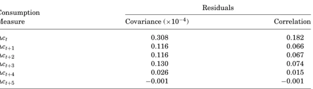
The table reports sample covariances and correlations between the innovation in montht’s log ex-cess aggregate stock return and innovations in contemporaneous and future log changes in real per capita consumption on nondurables and services. Innovations are residuals from OLS regressions on a set of instruments realized prior to the beginning of montht. The sample is 503 observations from February 1960 through December 2001.
Residuals Consumption
Measure Covariance (×10−4) Correlation
ct 0.308 0.182 ct+1 0.116 0.066 ct+2 0.116 0.067 ct+3 0.130 0.074 ct+4 0.026 0.015 ct+5 −0.001 −0.001
Consider then-month excess log stock return from montht−(n−1) to month
t,ni=−01rt−i. An ex post estimate of the covariance of this return with contem-poraneous consumption growth is
Cov∗ n−1 i=0 rt−i,ct+k−ct−n ≡ n−1 i=0 ˆ er,t−i−1,t−i−1,t−ieˆc,t−i−1,t−i−1,t−i+k. (43) If k is positive in (43), then consumption growth is measured over a longer horizon than returns, as discussed in the previous subsection.
This measure is not simply the product of the residuals of then-month stock return and the (n+k)-month log change in consumption. This latter product is also an ex post covariance estimate, but it does not take advantage of higher fre-quency data. An example will help clarify the difference between the measure in (43) and the product of multi-month residuals. Consider the case of quar-terly stock returns, orn=3. Then (43) is an ex post estimate of the quarterly covariance between returns and consumption growth that is constructed with monthly data.10For example, ifk=0, this estimate is the sum of the monthly ex post contemporaneous covariance estimates for each month in the quarter. The alternative ex post quarterly covariance estimate (ˆer,t−3,t−3,t)(ˆec,t−3,t−3,t) is effectively the sum of nine monthly ex post covariance estimates; the residual for each month’s stock return multiplied by the residual for each month’s con-sumption growth. Since the noncontemporaneous covariances should be zero withk=0, including them in the covariance estimate simply adds noise.
10Quarterly consumption growth here is defined as the log change from monthtto montht+3.
Because of time averaging this differs from the log change in average consumption during quarter τto quarterτ+1.
Multi-month estimates of the ex post variance of stock returns are defined analogously to the covariance estimate:
Var∗ n−1 i=0 rt−i ≡ n−1 i=0 ˆ er2,t−i−1,t−i−1,t−i. (44) The excess stock return fromt−n+1 tot(adjusted for Jensen’s inequality) is regressed on (43) using the instrument vectorZt−n:
n−1 i=0 rt−i+ 1 2Var ∗ n−1 i=0 rt−i =b0+[b1+b2pt−n]Cov∗ n−1 i=0 rt−i,ct+k−ct−n +wt. (45)
Ifn=1 in (45), we recover the single-period instrumental regression (20), or with a longer horizon for measuring consumption growth, (34).
In this paper I report results forn=1 (monthly returns) andn=3 (quarterly returns). In order to avoid overlapping observations withn=3, I estimate (45) on every third monthly observation. I choose the last month of each quarter. Since GMM estimation requires that this equation be estimated jointly with the zero-stage regressions, which are defined at a monthly frequency, I adopt the fol-lowing procedure. The zero-stage regressions used to construct monthly residu-als are estimated using just the last month of each quarter. Since construction of quarterly ex post variances and covariances requires residuals for each month in the quarter, the parameter estimates from these zero-stage regressions are then used to construct fitted residuals for all months in the sample.
Regressions of stock returns on higher frequency estimates of second mo-ments have a long history in finance, although applications have focused on estimates of stock return volatility. In spirit, the combination of (43) and (45) is similar to the procedure adopted by Whitelaw (1994). He uses the sum of squared daily aggregate stock returns to construct ex post estimates of longer horizon aggregate stock return volatility. He then uses an instrumental vari-ables setup to regress longer horizon returns on these volatility estimates.
IV. The Predictability of the Conditional Covariance
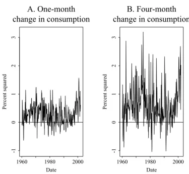
In this section I summarize the evidence from first-stage regressions in which ex post covariance estimates are projected on a set of instruments. Figure 3 dis-plays the time series of the ex post estimates. For Panel A, consumption growth is measured by the change in log consumption fromt−1 tot. For Panel B, it is measured by the change fromt −1 to t +3. The slow adjustment of con-sumption means that the latter measure produces ex post estimates that are both larger and more volatile than those produced with the former measure. The figure also shows that the outliers are more extreme when consumption growth is measured over the longer horizon. In particular, the observation for
Date Percent squared 1960 1980 2000 -10 0 1 0 20
A. One-month
change in consumption
Date Percent squared 1960 1980 2000 -10 0 1 0 20B. Four-month
change in consumption
Figure 3. Ex post estimates of the covariance between aggregate stock returns and consumption growth.The innovations to month-t’s aggregate excess stock return and per capita real consumption growth are constructed with OLS forecasting regressions. Consumption growth is measured with either the change from montht−1 to montht(Panel A) or from montht−1 to montht+3 (Panel B). The product of these innovations is an ex post estimate of the montht conditional covariance. The sample period is February 1960 through December 2001.
March 1980 is more than 8 standard deviations away from 0. This observation was driven by a particular event: the credit controls announced by the Carter administration in March. The stock market fell 12% in the month, while aggre-gate consumption fell dramatically through May before leveling off in June.11 The credit controls probably distorted investors’ first-order conditions. Conve-niently, this single observation generally has little effect on any of the results reported below. When there is an exception to this rule I note it.
Results from the first-stage regressions are displayed in Table III. In Panel A of the table, the horizon over which the covariance is measured is noted in the first column. Consumption growth is measured as indicated in the second column. The first four rows of Panel A report results for the entire set of in-struments itemized in (24). There is overwhelming statistical evidence against the null hypothesis of constant conditional covariances. For each horizon and consumption measure, the null hypothesis is rejected at less than the 1% level. TheF-statistics are similar in size to those used in the Monte Carlo simulation of Section III.A. The fitted values for the monthly regressions are displayed in Figure 4. In relative terms, there is substantial variation in the conditional