Feeling: sentiment analysis on Twitter

(1)

Computer Science and Engineering

Bachelor’s degree Thesis

Author: Sinclert Pérez Castaño

Directora: Lara Quijano Sánchez

(2)

Special thanks to:

Lara, my academic tutor for having patience with me and my irregular workflow. My English-speaking friends for correcting my not very academic English grammar while being abroad in California.

My parents, for supporting me every single moment. The completion of this Bachelor’s degree would not have been possible without them.

(3)

GENERAL INDEX:

0. ABSTRACT 8 1. INTRODUCTION 9 1.1. GENERAL OVERVIEW 9 1.2. PROJECT DESCRIPTION 10 1.3. MEMORY STRUCTURE 11

2. STATE OF THE ART 12

2.1. SENTIMENT ANALYSIS 12

2.1.1. TYPE OF PROBLEM 12

2.1.2. MAIN CHALLENGES 13

2.1.3. ACCURACY ISSUES 13

2.2. MACHINE LEARNING ALGORITHMS 14

2.2.1. LOGISTIC REGRESSION 14

2.2.2. BERNOULLI NAÏVE BAYES 15

2.2.3. LINEAR SUPPORT VECTOR MACHINE 15

2.2.4. RANDOM FOREST 17

2.3. RELATED PAPERS, BOOKS AND TUTORIALS 18

2.4. POSSIBLE TOOLS 20

2.4.1. ACCESSING TWITTER API 20

2.4.2. ANALYZING DATA 20 2.4.3. LEARNING ML MODELS 20 2.4.4. WEB FRAMEWORKS 21 2.4.5. FINAL DECISION 21 3. PROJECT OVERVIEW 22 3.1. MAIN OBJECTIVES 22 3.2. CLASSIFICATION DESCRIPTION 23 3.3. CLASSIFICATION SCHEME 24

(4)

4. DEVELOPED WORK 26 4.1. INTRODUCTION 26 4.2. APPLICATION ARCHITECTURE 27 4.2.1. MASTER BRANCH 27 4.2.2. SERVER BRANCH 28 4.3. KNOWLEDGE MODEL 29 4.3.1. MASTER BRANCH 29 4.3.2. SERVER BRANCH 32 4.4. EXECUTION DYNAMICS 34 4.4.1. TRAIN FUNCTIONALITY 34 4.4.2. SEARCH FUNCTIONALITY 35 4.4.3. CLASSIFY FUNCTIONALITY 36 4.4.4. STREAMING FUNCTIONALITY 37 4.5. USERS GUIDE 38 4.6. DEVELOPER GUIDE 40 4.6.1. EXECUTION COMMANDS 40 4.6.2. REQUIREMENTS 42

4.7. ESTIMATIONS AND PLANNING 43

4.7.1. ESTIMATION OF COSTS 43 4.7.2. POSSIBLE RISKS 44 4.7.3. PROJECT PLANNING 45 5. RESULTS 46 5.1. EVALUATION PROCEDURE 46 5.2. EVALUATION METRICS 47 5.3. FEATURE ANALYSIS 48 5.3.1. POLARITY COMPARISON 48 5.3.2. SENTIMENT COMPARISON 51 5.3.3. COMPARISONS CONCLUSIONS 53 5.4. ALGORITHMS ANALYSIS 54 6. CONCLUSIONS 55

(5)

7. FUTURE WORK 57

7.1. BACK-END IMPROVEMENTS 57

7.2. FRONT-END IMPROVEMENTS 58

(6)

I

NDEX OF FIGURES

FIGURE 2.1:SENTIMENT ANALYSIS APPROACHES ... 12

FIGURE 2.2:LOGISTIC REGRESSION ... 14

FIGURE 2.3:EXAMPLES DISTRIBUTED OVER SPACE ... 16

FIGURE 2.4:SVM KERNEL TRICK ... 16

FIGURE 3.1:HIERARCHICAL CLASSIFICATION ... 23

FIGURE 3.2:CLASSIFICATION SCHEME ... 25

FIGURE 4.1:MAIN BRANCH STRUCTURE ... 27

FIGURE 4.2:SERVER BRANCH STRUCTURE ... 28

FIGURE 4.3:WEB APP INTERFACE ... 38

FIGURE 4.4:ACCOUNT ANALYSIS INTERFACE ... 39

FIGURE 4.5:STREAM ANALYSIS INTERFACE ... 39

FIGURE 5.1:POLARITY MODEL WITH 1% UNIGRAMS ... 48

FIGURE 5.6:SENTIMENT MODEL WITH 1% UNIGRAMS ... 51

FIGURE 5.8:SENTIMENT MODEL WITH 3% UNIGRAMS ... 52

(7)

Index of Equations

EQUATION 2.1:LOGISTIC REGRESSION ... 14

EQUATION 2.2:BAYES RULE ... 15

EQUATION 2.3:SVM(A) ... 16

EQUATION 2.4:SVM(B) ... 16

EQUATION 2.5:GINI INDEX ... 17

EQUATION 2.6:ENTROPY ... 17

EQUATION 2.7:ERROR RATE ... 17

(8)

0.

Abstract

Nowadays, social networks contain information that can be used to extract knowledge from it, however, the insights from that information are usually accessible to companies but not to individuals. The aim of this project is to provide an accessible web application that makes use of Machine Learning algorithms together with Twitter official’s API to perform Sentiment Analysis over a set of tweets. Different natural language and feature engineering techniques have been applied to generate a range of trained models, including Logistic Regression, Bernoulli Naïve Bayes, Support Vector Machines and

Random Forest. Finally, these models have been compared to one another and several conclusions were drawn: Bernoulli Naïve Bayes and SVM performed the best, even if resulting in a F-score larger than 0.9, without suffering overfitting, is extremely difficult.

Actualmente, las redes sociales contienen información que puede ser utilizada para extraer conocimiento, sin embargo, las conclusiones de esa información son normalmente accesibles solo a las empresas, y no a los individuos. El objetivo de este proyecto es presentar una aplicación web que haga uso de algoritmos de Aprendizaje Automático junto a la API oficial de Twitter para realizar análisis de sentimiento en conjuntos de tweets. Diferentes técnicas de lenguaje natural y de ingeniería de características han sido aplicadas para obtener un conjunto de modelos, incluyendo

Logistic Regression, Bernoulli Naïve Bayes, Support Vector Machines y Random Forest. Finalmente, estos modelos han sido comparados entre ellos y varias conclusiones fueron obtenidas: Bernoulli Naïve Bayes y SVM son los modelos que mejor funcionan, considerando que obtener una F-Score superior a 0.9, sin sufrir sobreajuste, es extremadamente difícil.

(9)

1.

Introduction

1.1.

General overview

In the world we live, social networks are one of the main sources of personal information and interests across our daily lives. This is the reason why new sciences like “Social Network Analysis” and “Sentiment analysis” have become main fields of study and interest not only for the individual users but also for companies and governments. To get an idea of the amount of the data social networks, such as Twitter, store every day, it is enough to consider that each second around 6,000 tweets are generated (according to “Internet Live Stats”[1]), which give us around 500 million tweets per day. All these data contain information about very different topics and nature, so differentiating or analyzing very specific pieces of information across all the available resources is a powerful tool.

Sentiment analysis is a technique that is widely used in areas of social analysis research such as marketing, social networking development, reviews and survey responses, and especially in customer service. It uses natural language processing and text analysis to determine how an individual or group of people feel towards a specific situation. It can be also used to perform geolocation analysis such as political feelings (which political leader has better acceptance), marketing preferences (competitor’s products opinion over population) or, in general, any statistical analysis within the specified parameter.

Some real-world examples could be the analysis of the Brexit sentiment specified U.K. cities, or the acceptance of the new president of the United States throughout the different states.

This type of analysis can be used in respect to the social network Twitter and its “Application Programming Interface” (API). Twitter’s API is unique in the sense that it is easy to use, so anyone with basic programming knowledge can access large amounts of data in the form of tweets. Additionally, because of how people generally structure their tweets, most of them are solely comprised of plain text (unlike other social media platforms where users tend to include other media formats such as photos or videos), making them easier to analyze.

(10)

1.2.

Project description

The main goal of this project is to provide a simple sentiment analysis tool that can be used jointly with the Twitter API to classify tweets as “positive”, “negative” or “neutral”. The main differentiator factor with respect other Sentiment Analysis web application is that it is integrated with Twitter API, so automatic analysis over a certain account or a certain stream can be performed. Additionally, it is open to every individual user, not only to companies.

Although it was created relying on the previous introduced concepts, the project contains another important actor: Machine Learning (ML). ML includes a wide range of techniques that provides computers with the ability to learn without being explicitly programmed. Its use is not strictly necessary to perform a sentiment analysis task, because it could be done by simple human review, but for complex applications and tools in which large amounts of data are processed, it becomes the most common practice.

Machine learning plays a significant role in the data analysis processes because it helps to automate and generate a quicker response than the case of processing each piece of information (or tweet) individually by a person. In this project, ML techniques are used to classify tweets obtained through the Twitter API with one of the possible labels:

positive, negative or neutral.

Obviously, the application of ML algorithms does not guarantee an error reduction with respect to the individual processing case, however, the advantages due to the time performance and effort improvements make it worth. In this project, several algorithms will be tested and compared with each other to understand why some models perform better than others and which features are the best ones to consider (“feature engineering”). Testing them will be one of the core sections of this memory because improving the ML predictions on unclassified data will suppose a general improvement in the behavior of the application.

Finally, as a way of making this project more accessible in case of using a web domain to host it, the project contains a web-application structure so it can be used thought any internet browser.

In conclusion, this bachelor’s thesis consists of a web application that uses trained ML models to perform a sentiment analysis over a set of Twitter data specified by the user. The trained models need to be generated before the classification task, using a series of data sets obtained from a Python package called Natural Language Toolkit (NLTK).

(11)

1.3.

Memory structure

The memory document is structured as follows:

• Information about sentiment analysis papers and tutorials, why they are relevant, and some useful tools and ideas to apply in a project like this (point 2).

• A big overview of the main objective of the application (point 3).

• A detailed explanation about the component and technologies behind the application, why I have chosen those and how do they work (point 4).

• Testing and comparison of the different ML algorithm and cases with the obtained conclusions (points 5 and 6).

• A brief specification of the possible future work in case the work on this project is continued (point 7).

(12)

2.

State of the Art

2.1.

Sentiment Analysis

Sentiment analysis is a technique that determines the attitude of a person or group of people towards a certain product, situation or event. The premise is that all opinions can be classified in different groups (“positive”, “negative”, “neutral” …), each of them grouping several mood states. For example: sadness and anger belong to negative.

2.1.1.

Type of problem

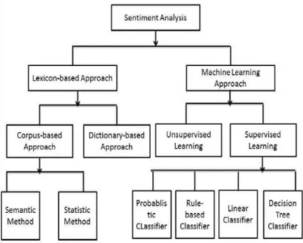
The main goal is to correctly classify the units of information (tweets) into one of the three aforementioned groups. It is considered a classification problem that can be approached using different methodologies, as this graph [2] shows:

Figure 2.1: Sentiment Analysis approaches

This project focuses on the ML branch because it is the most commonly used and the most popular because of nowadays trend. Some of the most relevant ones are the Naïve Bayes (NB) and the Support Vector Machine (SVM) classifiers, under the “Supervised Learning” category, which will be explained and analyze later on.

This classification problem may also be included under the “Unsupervised Learning”

category if there is no labeled data available. However, due to the amount of data not only in Twitter, but also in other social networks and web pages such as Amazon or eBay, it is not difficult to obtain datasets labeled with the Likert scale those e-commerce pages use. They can be found, for instance, in Kaggle.com.

(13)

The training data have been obtained from the NLTK corpus, where there are files containing neutral-polarized and negative-positive sentences. The downloaded files from the corpus are: sentence_polarity (containing 5,331 negative and 5,331 positive examples) and subjectivity (containing 5,000 neutral and 4,985 polarized examples). These examples are just sentences of different lengths that have been previously identified by their sentiment.

2.1.2.

Main challenges

Probably the most difficult part of the classification process is to differentiate between subjective tweets, which can be classify as positive or negative, and objective ones, which are considered as neutral. The subjectivity usually depends on the context so the units of information should be understood in the context of a conversation or in a sequence of them if the talk about the same topic.

On top of that, the utilization of sarcasm while writing an opinion make extremely difficult for the classifiers to detect it. This would not be that important if the percentages of comments using sarcasm remain low, however, due to the Twitter length limitation to 140 characters, users usually write in more creative ways than in others social networks, increasing the use of it.

2.1.3.

Accuracy issues

Due to the difficulties stated in the previous part, reaching an accuracy close to 100% is practically impossible. Even more, according to this sentiment analysis article [3], human judgement accuracy is around 79%. Because of this, if a specific software were right 100% of the times and we review the classified examples, we will still disagree with the program around 20% of the time.

These facts imply 2 things:

1. If a model, using any of the techniques of the Figure 2.1,achieve an accuracy rate higher than 79%, we could state that it is better than an average person trying to classify tweets into the polarity labels.

2. The complexity of achieving a high accuracy rate is extremely high, so the conclusions extracted from a sentiment analysis over a certain entity should always consider a margin of error.

(14)

2.2.

Machine Learning algorithms

The algorithms used during the development of this project have been chosen due to their flexibility. These algorithms are:

1. Logistic Regression. 2. Bernoulli Naïve Bayes.

3. Linear Support Vector Machine. 4. Random Forest.

2.2.1.

Logistic Regression

The idea behind this machine learning approach is to use a vector of weights called “θ” as long as the number of features. It could be described as a linear regression vector of weights, applying them into classification. Although this discriminative algorithm was designed to classification problems in which the number of possible classes is two, there exist an alternative for the multiclass problem (Soft-Max)[4][5].

The labels or classes are separated from each other using a hyperplane, which express the area of the features space with maximum confusion.

In order to obtain a classification result from the set of classes given a numeric result (multiplying the weights vector and each vector of features values), a Logistic sigmoid

function is applied. This function computes the probability of a particular instance to be considered as one or the other class.

Figure 2.2: Logistic Regression

(15)

2.2.2.

Bernoulli Naïve Bayes

There exist a group of ML algorithms that rely on probabilities. All of them are possible thanks to the “Bayes Rule” (explained later), in which knowledge can be obtain from a set of available labeled instances.

Inside the family of pure probabilistic approaches, there are two main models: the

Gaussian and the Bernoulli. The different between both of them is that the first one is considered a generative model, predicting a specific feature value (Xi) from the class that

example belongs to (y); and the second one is a discriminative model, in which the class is predicted using the vector of features [4][5].

Considering the type of classification task in which the project is based on, the only useful approach is the discriminative one (Bernoulli), because we will try to predict the sentiment feeling (class) of a text.

The Bernoulli Naïve Bayes, as its own name indicates, makes the naïve assumption of supposing that each feature is independent to the rest. Additionally, it uses Bayes rule

to compute the probability of each class:

𝑃 𝑦 𝑥 = 𝑃 𝑥 𝑦 ∗ 𝑃(𝑦)

𝑃(𝑥) Equation 2.2: Bayes rule Where:

• P(y|x) = the probability of belonging to class “y” giving the features “x”.

• P(x|y) = the probability of features “x” given “y”.

• P(y) = the total probability of the class “y”.

• P(x) = the probability of the vector ”x” (ignorable because is a global constant).

2.2.3.

Linear Support Vector Machine

The Support Vector Machines (SVM) are one of the most powerful ML algorithms due to their flexibility and good optimization. Additionally, thanks to the “kernel trick” technique in which more features are created almost free to expand the feature space, the classification errors are often reduced [4].

The basic idea is to create a linear boundary between examples belonging to different classes with the biggest possible gap (δ) between the closest examples to that line

(quadratic problem). Those points are called “support vectors” and they give the name to the model.

(16)

As Logistic Regression, it also uses a vector of weights (“w”), following these formulas in the case of binary classification:

A) When the class is 1: 𝑤 ∗ 𝑥* + 𝑏 ≥ δ

Equation 2.3: SVM (A) B) When the class is -1: 𝑤 ∗ 𝑥*+ 𝑏 ≤ -δ

Equation 2.4: SVM (B)

Due to some mathematical optimizations, it is possible to define that vector of weights as a weighted sum of support vectors. In conclusion, the linear boundary only depends on the closest examples to the itself, which are the ones defining the supporting vectors. Finally, the “Linear” nature of the SVM that I am describing is not because of the linear boundary, but because of how the “kernel trick” function is defined. This function is just a way of creating new features with the ones we already have and expand the features space so the boundary can easily differentiate among the classes [6].

Example: we want to classify the following examples:

Figure 2.3: Examples distributed over space

However, there is no clear linear boundary, so a “kernel trick” should be used to add 1 more dimension to the features:

Figure 2.4: SVM kernel trick

(17)

2.2.4.

Random Forest

The last considered ML algorithm in this project is based on decision trees. These trees are just connected nodes in which one of the features is evaluated, and depending on the result, different branches are taken. At the very end of the tree there are leaves, which are nodes containing the designated class [4][5].

The criteria to create the tree depends on the defined impurity function, which is going to determine when a specific node must be split into different ones and when that node is a leave. There exist several impurity functions for the binary classification problem: Given (𝑝 = 𝑛₁ 𝑛 ), and (𝑞 = 𝑛₃ 𝑛 ), where “+” and “-“ are the two classes:

• Gini index: 2 · 𝑝 · 𝑞

Equation 2.5: Gini index

• Entropy: −𝑝 · 𝑙𝑜𝑔 𝑝 − (𝑞 · 𝑙𝑜𝑔 𝑞 )

Equation 2.6: Entropy

• Error rate: 1 − max[𝑝, 𝑞]

Equation 2.7: Error rate

The main problem with decision trees is that, if no additional technique is applied when creating them, they tend to overfit. That is why popular approaches as pruning and trees combinations (Random Forest) started appearing.

A Random Forest is just a combination of decision trees, in which for each of them a small random features subset is used. Then the outputs of all these trees are combined to select the most popular class, a technique known as bagging.

(18)

2.3.

Related papers, books and tutorials

From the set of public papers, books and sentiment analysis tutorials available on the subject, the ones that proved to be the most useful throughout the project are the following:

• Twitter Developer Documentation [7]:

This is the official Twitter documentation about how their Application Programming Interfaces (APIs) work. There is information not only about how to make requests, but possible obtained data after each type of request.

Some of the most important data fields composing each tweet are:

• Coordinates

• Creation date.

• Entities (hashtags, URLs and user mentions).

• Favorite counter. • Retweet counter. • ID. • Language. • Place. • Possible sensitivity. • Text. • User.

However, there exist some statistics that can be obtained using the Twitter interface which cannot be obtained using its API: the number of views, and the number of engagements. Both would have been helpful to determine the importance of the retrieved tweets.

• Twitter Sentiment Analysis: A Review [3]:

This paper contains a general overview about the use of sentiment analysis with Twitter using ML algorithms to predict the labels. It also contains a brief explanation of the feature selection process: case normalization, tokenize, stop words (those without any important significance), stemming…

• Sentiment Analysis of Twitter Data [8]:

This one contains information about another sentiment analysis study in which they compare the use of different features and different algorithms to compare the results and extract conclusions. It is relevant because the use of Part of Speech (POS) tags is well explained.

(19)

• The Importance of Neutral Examples for Learning Sentiment [9]:

Paper that contains a detailed explanation about why the neutral class cannot be ignored when doing a sentiment analysis.

• Machine learning and Text Mining slides [5]:

Slides that contains information about ML algorithms and how they work, along with concepts descriptions. In terms of Text Mining, explanations and examples.

• Sentiment Analysis in Python [10]:

Online tutorial that describe the process of training a ML model in the Python programming language, along with example of feature selection. It also contains some links to other resources and tutorials in which this one is based on, that were useful during the development of the project.

• Twitter Sentiment Analysis with NLTK [11]:

Online tutorial that explains in a series of videos with supporting code examples the different possibilities of NLTK and the learning algorithms available inside the NLTK package. Although none of the NLTK algorithms were used in this project, the videos were helpful to understand some of the package capabilities.

(20)

2.4.

Possible tools

There exist a large list of possible tools and technologies that are publicly available to perform a ML approach into the sentiment analysis of Twitter data. Each of these classification process stages is going to be considered independently in order to explain the different options in each of the cases.

2.4.1.

Accessing Twitter API

In this case, there are not a lot of options because there exist only one official Twitter API. However, there exist several libraries and packages across different programming languages to make our communication with the API easier.

There exist libraries for several programming languages such as Java, Python, Objective-C, C++, Go, PHP and Ruby, although only Java and Python were considered at the end. The full list can be consulted in the Twitter developer’s documentation, under the

Twitter libraries category [12].

These libraries allow developers to access a wide list of information fields associated to each individual tweet, making possible to create statistic analytical tools as the one described here. Some of the information fields are: coordinates, creation date, entities, number of favorites, number of retweets, language, place, possible sensitive, user…

2.4.2.

Analyzing data

The following pieces of software can help on two different processes: cleaning the tweets obtained from the API, and processing the training examples using Natural Language Processing (NLP) techniques to select the most informative features that the ML models will use to learn later.

• Python Natural Language Toolkit (NLTK) package.

• Java Stanford CoreNLP library.

2.4.3.

Learning ML models

After the data analysis, a model must be trained to predict the classification label of future tweets. There is a big range of options, because even the NLTK contains its own classification module, but there exist more specialized libraries such as:

• Java Weka library.

• Java General Architecture for Text Engineering (GATE) library.

• Python Scikit-learn package.

(21)

2.4.4.

Web frameworks

Finally, with the aim of providing web characteristics, a framework to connect the Back-end consisting on the trained model and the Front-Back-end was required. The libraries listed below were considered for their simplicity since the project’s web behaviors does not required complex functionalities. They are all Python frameworks:

• Python Django

• Python Web2py

• Python Flask

2.4.5.

Final decision

Due to the extended documentation of “Tweepy” (3.5 version), “NLTK” (3.2 version) and “Scikit-learn” (0.18 version) packages, the Python programming language was used to implement the project combining the functionalities of these packages. Moreover, they have open source licenses so they can be used to academic projects but not commercial software.

Additionally, “Flask” (0.12 version) micro framework was used to create the web infrastructure. This framework is preferable over Django or Web2Py because it provides more direct control over the project structure and communication.

All these packages provide already implemented functions that make the development process easier, because they provide a solid base in which start building the logic that will shape the functionality of the software. Moreover, there are some of the Scikit-learn

algorithms that have been incredibly optimized using C code, and a possible pure Python implementation will almost certainly be slower.

During the development process PyCharm, which is a very complete development environment, was used along with a GitHub repository, where all the changes have been submitted. Thanks to the version control in this last platform, the code can be diverged in different work flows called “branches”, that will be necessary in the future (further explanation in section 4.1).

(22)

3.

Project overview

This overview contains explanations about the project goals, how the project classification challenge has been approached and its general steps. There is a need for explaining the chosen approach because it does not follow the standard classification procedure.

3.1.

Main objectives

The main objective is to build a software tool which performs sentiment analysis over pieces of information in the shape of tweets, and that it is accessible to everyone. Accessible meaning a free, and easy to use and web application (once the project is hosted) that any individual can use without previous knowledge.

A good example of its usage is to determine the feeling of citizens in a certain city over a specific political party, brand, law…

In order to achieve that functionality, a Twitter API text mining implementation for tweets extraction is required. The retrieved data can be used either to perform the analysis specified by the user or to expand the datasets used in the feature engineering process and in the ML models training.

After the data has been retrieved, the goal was to build a feature engineering function to get the most relevant features of each piece of information. This is a crucial step in the project because feature selection has a big effect in the final score of ML classifiers. Additionally, obtaining an insight in the algorithms performance in the case of text classification was one of the goals. It is possible thanks to the use of ML algorithms such as Logistic Regression, Naïve Bayes, Support Vector Machines, and Random Forest as well as the manual modification of their parameters.

In terms of software, the project was designed to embody the following characteristics:

• Accessible: any individual with internet connection can use it.

• Effective: as much as possible due to the M.L. classification errors.

• Fast: it needed to be fast enough to later be transformed into a web application.

• Easy to use:no previous knowledge required.

(23)

3.2.

Classification description

When considering classification problems, the most popular technique to approach them is by discriminative models. These models predict the class (y) of a new instance (x). Some of the models use a probabilistic approach (Naïve Bayes) and some others just a linear boundary (Logistic Regression or Support Vector Machines), both of them have the same goal: to predict the correct class (or label).

In Sentiment Analysis, three possible classes exist: “neutral”, “negative” and “positive”, however, not all of them have the same relationship among each other. Although the labels “negative” and “positive” have an intrinsic relationship in which one is the opposite of the other, that is not the case with “neutral”. When discussing text classification, the opposite to “neutral” is “polarized”.

Due to the unbalanced relationship among the possible classes, the method to classify the tweets is not going to be a common classification over three labels. Instead, it will be a hierarchical classification over two possible labels (“neutral” and “polarized”), and depending on the outcome, between the other pair of them.

Therefore, the classification process is as follows:

Figure 3.1: Hierarchical classification

This way, each label shares the same hierarchical level as its opposite and the classification process is more balanced. The main problem when including a hierarchical structure is that the errors from the first classifier affect the second one.

(24)

3.3.

Classification scheme

In order to have a global overview of the classification scheme, the taken sequence of steps are shown:

1. Open the data files containing the raw sentences expressing sentiment. They have been obtained using the NLTK corpus, and the sentences are organized in 4 different text files: Neutral, Polarized, Negative and Positive.

Neutral example: “There has been an attack in London, according to CNN”

Polarized example: “I believe they can win the next championship” Negative example: “Cleveland could have done more! so sad”

Positive example: “Morning! today is a nice day in the bay!”

2. Clear the sentences: tokenize them, converting all the words to lower case; remove the stop words (list of non-informative words obtained from the NLTK corpus to filter the sentences); and lemmatize the remaining ones. After doing this, we can obtain a list of words and a list of bigrams (sequences of 2 words). Clean neutral: [“there”, “attack”, “London”, “according”, “CNN”] Clean polarized: [“believe”, “win”, “championship”]

Clean negative: [“Cleveland, “more”, “sad”]

Clean positive: [“morning”, “nice”, “day”, “bay”, “nice day”]

3. Feature selection using NLTK functionalities. The best results have been obtained using the Chi-Square distribution to get the scores of words and bigrams, and selecting the best of them.

Informative words [… , “there”, “according”, “believe”, “sad”, “nice”, ... ] Informative bigram: [... , “nice day”, ... ]

4. Transform the dictionary of features into a vector using Scikit-learn modules. Neutral features: {… , “there”: 1, “according”: 1 , … ]

Polarized features: {... , “believe”: 1, ... } Negative features: {... , “sad”: 1, ... }

(25)

5. Train the different models with pairs of training examples: Neutral – Polarize, and Negative – Positive. After comparing the results (in section 5.4), the model with higher combined accuracy is selected and stored in the Models folder. 6. On the web part, tweets are obtained using the Twitter API, and they are cleaned

and vectorized, just as the data files sentences.

7. Finally, the best models are loaded into memory and the tweets are classified, both in the case of a user account and the streaming tweets.

(26)

4.

Developed work

4.1.

Introduction

The project was started as a local Python program in order to test the viability of the initial idea. Later, the code was separated into two different branches using GitHub to improve version control.

The first branch has a local scope, in the sense that it is thought to be executed in the local machine of the user that wants to operate with it, instead of using the software through the browser as a web application. The possible functionalities that are available in this branch are the following:

• Train models: L.R. / Bernoulli N.B. / Linear S.V.M. / R.F.

• Search for tweets to increase the size of the training datasets.

• Classify tweets of a user filtered by a word as neutral, positive or negative.

• Visualize a stream of tweets filtered by word and coordinates.

The second branch is a modification of the first one, in which other files such as the HTML, CSS and JavaScript have been included. Once the program is executed simulating a hosted web app, the functionalities are reduced to the following two:

• Classify tweets of a user filtered by a word as neutral, positive or negative.

• Visualize a stream of tweets filtered by word and location.

The reason why the first branch is relevant to the project and it has been kept instead of having just the second branch, is because it can be used to generate the models that can be moved to the second branch folder structure and use them. Additionally, almost all the debugging over the text processing, features selection, and model’s accuracy comparison, have been done with that code.

From the final user perspective, only the second branch is useful once the best possible model has been selected and generated, because is the one containing the web functionalities, however both are important.

(27)

4.2.

Application architecture

4.2.1.

Master branch

The main branch is structured into the following files and folders: A) Files:

• Classifier: contains a class with the functions to train, obtain the features of a text, save and load the models.

• DataMiner: contains the class with the functions to obtain tweets from a specified user or in general, filtering with some parameters.

• GraphAnimator: contains a function to display the results of the stream.

• Keys: contains the app and administrator (me) keys to access the API.

• Parser:contains the functions to parse the user arguments and execute the indicated functionality.

• TwitterListener: contains a class with the methods to initiate the stream, handle the obtained tweets and close the stream.

• Utilities: contains several functions that are useful across different functionalities and files.

B) Folders:

• Datasets: contains the data files used to train the models.

• Models: is the folder where the trained models are going to be stored.

(28)

4.2.2.

Server branch

The server branch is structured into the following files and folders: A) Files:

• Classifier: contains a class with the functions to train, obtain the features of a text, save and load the models.

• DataMiner: contains the class with the functions to obtain tweets from a specified user or in general, filtering with some parameters.

• Keys: contains the app and administrator (me) keys to access the API.

• Parser:contains the functions to parse the user arguments and execute the indicated functionality.

• Server: contains the associated functions to web directions.

• TwitterListener: contains a class with the methods to initiate the stream, handle the obtained tweets and close the stream.

• Utilities: contains several functions that are useful across different functionalities and files.

B) Folders:

• Datasets: contains the data files used to train the models.

• Models: is the folder where the trained models are going to be stored.

• Stopwords: contains the files with the stop words in different languages.

• Static: contains the static web files such as CSS, JavaScript, images…

• Templates: contains the HTML files.

(29)

4.3.

Knowledge model

In this section, every function in the code is described. However, those that belong to a specific class are going to be covered under their class definition.

4.3.1.

Master branch

CLASSIFIER

Type: Python - Class

Description: Represents a classification model.

Parameters: • Tokenizer: object that separate words in a text.

• Vectorizer: object that transform features into a vector.

• Lemmatizer: object that obtain words lemma (root).

• Stopwords: list of stop words of the given language.

• Model: object containing the trained model.

• Best_words: list of most informative words.

• Best_bigrams: list of most informative bigrams.

Functions: • getWords: obtains a list of filtered words in a sentence.

• getWordsAndBigrams: obtains a list of all filtered words and bigrams in the specified file.

• getFeatures: obtains a dict. of features given a sentence.

• performTraining: trains the model and prints its accuracy.

• train: obtain the training data after several function calls.

• classify: classify a sentence after obtaining its features.

• saveModel: save the model in a pickle file

• loadModel: load a model from a pickle file

DATA MINER

Description: Mining object that extract data from Twitter API.

Parameters: • API: object that contains the API connection to Twitter. Functions: • getUserTweets: gets user tweets, optionally filtered.

• searchTweets: stores in a text file the tweets that fulfill the specified query conditions.

(30)

GRAPH ANIMATOR – ANIMATE PIE CHART

Type: Python - Function

Description: Graph generator to visualize the results from the Twitter listener streaming, using Matplotlib.

PARSER

Type: Python - Executable file

Description: Executable containing the argument parser for the different project functionalities.

Parameters • Dataset folder: folder name where the data is stored.

• Models folder: folder name where the models are stored.

• Labels: labels among which classification is performed. Functionalities: After parsing the received argument, select one of the following:

• Train: trains and saves a model.

• Classify: prints the classifications results after loading a trained model.

• Search: extracts tweets and stores them into a text file.

• Stream: starts a streaming sharing a data structure with the GraphAnimator function.

TWITTER LISTENER

Description: Object taking control of each Twitter streaming API.

Parameters: • API: object that contains the API connection to Twitter. Functions: • updateBuffers: updates a circular buffer that store the

last “n” classifications results.

• initStream: initiates the stream with the provided args.

• closeStream: closest the stream.

• on_status: process each received tweet (overrides).

(31)

UTILITIES – GET STOP WORDS

Description: It gets all the stop words defined in the specified language text file inside the “Stopwords” folder, and return them as a list.

UTILITIES – GET BEST ELEMENTS

Description: It performs a statistical distribution analysis using the Chi-square

test to select the most informative features given two sets of features in the form of Counters.

UTILITIES – GET CLEAN TWEET

Description: It obtains the text from a tweet object, without all the entities that are not considered text (user names, hashtags, links…)

UTILITIES – GET SENTENCES

Description: It split a given text into sentences returning them as a list.

UTILITIES – STORE TWEETS

Description: It stores the list of tweets received as argument in the specified text file.

(32)

4.3.2.

Server branch

This section contains the description of the new functions introduced in this branch of the code. Some of them are not included because they are exactly the same as the ones in the main branch.

All the Back-End functionalities are inside the Server file. Additionally, there is a web structure composed by a HTML, a CSS and a JavaScript (JS) file.

GRAPH.JS

Type: JavaScript

Description: Contains the JS functions used to animate the web page and communicate with the Python Back-end.

Parameters: None.

Functions: • ready: links JS functions to web page buttons.

• toogleAccount: hides the “stream” lateral bar section, showing the “account” one.

• toogleStream: hides the “account” lateral bar section, showing the “stream” one.

• showAbout: shows a section in the middle of the web page containing information about the author.

• hideAbout: hides the section in the middle of the page.

• accountRequest: performs a HTTP request to Back-End, showing a loading wheel while waiting.

• streamRequest: performs a HTTP request to Back-End to initiate the stream, and then one each 750 ms.

• showLoading: shows the loading wheel.

• hideLoading: hides the loading wheel.

• getCoordinates: gets coordinates of the location the user has specified using Google geocode API.

• finishStream: stops the stream sending a HTTP request.

• accountHandler: updates the pie with the response.

• streamHandler: updates the pie graph with the response.

• updatePie: updates the pie graph with the new counters.

• createPie: create a pie graph in case of not having one.

• showError: shows and error in the center of the screen.

(33)

SERVER

Type: Python – Back end

Description: Contains the different Flask functions callable from the front end (through HTTP requests).

Parameters: None.

Functions: • index: loads the classifiers and renders the index.html.

• classifyAccount: classifies the tweets contained the filtering word of the specified user, returning the counters as a json.

• initStreaming: initiates a Twitter streaming.

• endStreaming: finishes the Twitter streaming.

• streaming: returns as json the results of the Twitter streaming buffer (classification counters).

• getAPI: generates an API connection with Twitter. It can be application or user type.

(34)

4.4.

Execution dynamics

All the previously detailed functions need to work together to provide some functionalities. All the following ones are available to the developer behind the project, but only two of them (“classify” and “Streaming”) are accessible to the final users through the web application.

4.4.1.

Train functionality

In this functionality, the input strings are parsed using the Parser.py file, creating a Classifier object, and calling:

1. Method train:

• Inputs:

- Classifier name (string). - First dataset name (string). - Second dataset name (string).

- Percentage of words to use as features (integer). - Percentage of bigrams to use as features (integer).

• Outputs: -

• Calls:

1.1. Method getWordsAndBigrams (x2):

• Inputs: dataset path (string).

• Outputs:

- Dataset sentences (list of strings). - Dataset words (counter of strings). - Dataset bigrams (counter of strings).

• Calls:

1.1.1. Method getWords:

• Inputs: sentence (string).

• Outputs: sentence words (list of strings).

1.2.Method getBestElements:

• Inputs:

- First dataset elements (counter of strings). - Second dataset elements (counter of strings). - Percentage of them to keep (integer).

(35)

1.3. Method getFeatures (x2):

• Outputs: features (dictionary of words and bigrams).

• Calls:

• Outputs: sentence words (list of strings).

1.4.Method performTraining:

• Inputs:

- Classifier name (string).

- Features (sparse numpy matrix). - Labels (numpy array).

• Outputs: -

2. Method saveModel:

• Inputs:

- Models folder name (string). - Output model name (string).

• Outputs: saved “pickle” file.

4.4.2.

Search functionality

In this functionality, the input strings are parsed using the Parser.py file, creating a DataMiner object, and calling:

1. Method searchTweets:

• Inputs:

- Filter query (string). - Language (string). - Storing file path (string). - Depth (integer).

• Outputs: -

• Calls:

1.1. Method getCleanTweet:

• Inputs: tweet (object).

(36)

4.4.3.

Classify functionality

In this functionality, the input strings are parsed using the Parser.py file, creating a DataMiner object, and calling:

1. Method getAPI (only in Server branch):

• Inputs: connection type (string).

• Outputs: Twitter API (object).

2. Method getUserTweets:

• Inputs:

- User name (string). - Filter word (string). - Depth (integer).

• Outputs: tweets (list of strings).

• Calls:

1.1. Method getCleanTweet:

• Outputs: clean tweet text (string).

3. Method getSentences:

• Inputs:

- Tweets (list of strings). - Filter word (string).

• Outputs: sentences (list of strings).

• Calls: getSentences (recursive).

4. Method classify (x2):

• Outputs: predicted label (string).

• Calls:

3.1. Method getFeatures (x2):

• Outputs: features (dictionary of words and bigrams).

• Calls:

(37)

4.4.4.

Streaming functionality

In this functionality, the input strings are parsed using the Parser.py file, creating two Classifier objects, and calling:

1. Method getAPI (only in Server branch):

• Inputs: connection type (string).

• Outputs: Twitter API (object).

2. Method loadModel (x2):

• Inputs:

- Models folder (string). - Model name (string).

• Outputs: -

3. Method initStream:

• Inputs:

- Query (string). - Language (string).

- Coordinates (string of four floats separated by commas).

• Outputs: -

• Set listeners:

2.1. Method on_status:

• Inputs: tweet (object)

• Outputs: -

• Calls:

2.1.1. Method getCleanTweet:

• Outputs: clean tweet text (string).

2.1.2. Method updateBuffers:

• Inputs: label (string).

• Outputs: -

2.2. Method on_error:

• Outputs: -

4. Method animatePieChart (only in Master branch):

• Inputs:

- Labels (list of strings). - Tracks (string).

(38)

4.5.

Users guide

From the point of view of the user, the interaction with the project is going to be through a web browser. In order to make this possible, all the project files need to be hosted by a service such as, Google Cloud or Heroku. Even if the final deployment in a hosting service does not take place, this guide will still be useful once the project is deployed. The main and single page of the web application is like this:

Figure 4.3: Web app interface The interface is divided in the following sections:

1. Header: shows information about the tool. The title and a brief description of what the application does.

2. Options: a pair of buttons to select the functionality of the tool. Each of them requires different input fields to be fulfilled by the user.

A) Account: classify the tweets from an account. B) Streaming: classify live tweets from a location.

3. Input fields: contains the fields the user needs to provide to start the analysis. They change depending on which functionality is selected.

4. Content: shows the pie chart once it is generated.

(39)

Figure 4.4: Account analysis interface

Figure 4.5: Stream analysis interface

Where:

6. Account field: where the Twitter account is specified (without the “@” symbol).

7. Filter field: where the word used to filter the tweets is specified.

8. Graph: it contains the classification categories represented as a pie chart.

9. Graph legend: interactive legend whose labels can be removed or added.

10. Region field: where the city or region to filter the stream of tweets is specified.

(40)

4.6.

Developer guide

This guide is designed for developers working with this project in the future. It contains information about how to execute both branches and system requirements.

4.6.1.

Execution commands

The Master branch is designed to be executed locally to refined the feature selection and ML model. Additionally, it could be used to increase the training dataset by searching tweets, and check the functionalities of the web-application, which are: classify account tweets and classify tweets from a stream.

The way to execute this project branch is with the “Parser.py” file:

Where the list of functionalities with their group of arguments are:

1. Train a Machine Learning model:

Functionality: “Train” Arguments:

A) Classifier: “Logistic-Regression”, “Naive-Bayes”, “Linear-SVM” or

“Random-Forest”.

B) File 1: name of the first file inside “Datasets” folder used to train. C) File 2: name of the second file inside “Datasets” folder used to train. D) Words percentage: percentage of total words used as features. E) Bigram percentage: percentage of total bigrams used as features. F) Output: name of the output classifier to store in “Models”.

Example:

2. Search for Tweets:

Functionality: “Search” Arguments:

A) Query: sequence of words to filter the search.

B) Language: language in which the retrieved tweets are. C) Depth: number of tweets that we want to retrieve.

D) Output: name of the output dataset to store in “Datasets”. Example:

$> python Parser.py <Functionality> <List of arguments>

$> … Train Logistic-Regression Positive.txt Negative.txt 5 1 Pos-Neg

(41)

3. Classify tweets from an account:

Functionality: “Classify” Arguments:

A) Polarity model: name of the model to differentiate neutral and

polarized sentences, stored in “Models” folder.

B) Sentiment model: name of the model to differentiate Positive and Negative sentences, stored in “Models” folder.

C) Account: Twitter account whose tweets are going to be classified. D) Filter word: word or sequence of words used to filter the tweets. Example:

4. Classify tweets from a stream:

Functionality: “Stream” Arguments:

A) Polarity model: name of the model to differentiate neutral and

polarized sentences, stored in “Models” folder.

B) Sentiment model: name of the model to differentiate Positive and Negative sentences, stored in “Models” folder.

C) Buffer size: number of most recent tweets to consider in the chart. D) Filter word: word or sequence of words used to filter the tweets. E) Language: language in which the tweets are filtered.

F) Coordinates: sequence of 4 float numbers separated by commas that indicates the southwest and the northeast corners of the region delimiting where the tweets are retrieve.

Example:

Even if the provided implementation does not use all the possible arguments a Twitter Stream can take, the whole list of them can be checked in the official Twitter documentation [13].

As for the Server branch, the python file to run is called “Server.py” with no arguments. Note that it may take a few seconds before the server is operational.

The way to execute this project branch is with the “Server.py” file:

$> … Classify Neu-Pol Pos-Neg David_Cameron Brexit

$> … Stream Neu-Pol Pos-Neg 500 Obama en -122,36,-121,38

(42)

4.6.2.

Requirements

The system requirements in this section are just software requirements. The project requires a specific version of the Python interpreter alongside a series of Python packages that have been used during the development.

Any package dependencies are state under their names:

• Python interpreter: Python 3 (v3.4 or superior)

• Packages: o Tweepy (v3.5 or superior) § Six (v1.10 or superior) § Requests (v2.14 or superior) § Requests-oauth (v0.8 or superior) o NLTK (v3.2 or superior) § Six (v1.10 or superior) o Scikit-learn (v0.18 or superior) o Numpy (v1.12 or superior) o Flask (v0.12 or superior) § Werkzeug (v0.12 or superior) § Jinja2 (v2.9 or superior) § Click (v6.7 or superior) § Itsdangerous (v0.24 or superior)

(43)

4.7.

Estimations and planning

4.7.1.

Estimation of costs

In this section, the software development costs of this Bachelor’s degree thesis are going to be estimated. Physical, indirect and human resources during the nine months of development are going to be detailed. All the costs have been calculated without taxes.

• Physical resources:

The physical resources associated with the software development are basically technical because of the nature of the project. The cost related with the future hosting have not been included.

Resource Quantity Cost

MacBook Pro 13’’ 1 1,445 €

PyCharm license 1 159 €

Microsoft Office 365 license 1 70 €

• Indirect resources:

All the costs related with the completion of the project but that cannot be considered key project development tools are considered indirect costs.

Resource Cost per month Months Cost

Internet 30 € 9 270 €

Electricity 40 € 9 360 €

• Human resources

Given that the development has been done by one person and supposing a salary of 9€ per hour, the cost of human resources are as follows:

Phase Salary per hour Hours Cost

Software project 9 € / h 350 4,050 €

(44)

• Total costs: Concept Cost Physical resources 1,675 € Indirect resources 630 € Human resources 5,670 € TOTAL 7,975 €

4.7.2.

Possible risks

There exist some risks related with the correct deployment and functionality of the software tool. Most of these risks are external circumstances to the software that is provided in the link of section 4.1.

• Incompatibilities among the different used packages:

As the explained software project use several Python packages to provide a more complex functionality, the upgrade of those packages could produce incompatibilities among them, leading to an error when trying to execute any of the functionalities (train a model, search for tweets, classify tweets of an account, classify tweets of a stream).

• Web application hosting server down:

In case of hosting the web application in a hosting service such as Google Cloud

or Heroku, the software is not going to work if the hosting server goes down. The only recommendation to avoid this risk is to select a good hosting service that could guarantee a certain minimum of time up.

• Impossibility of increasing the datasets with new examples:

When using the Search functionality to try to increase the training datasets, it is not always easy to find relevant and informative tweets for the desired sentiment. Moreover, as the project uses the Twitter official API, the retrieved tweets could suffer bias depending on how Twitter retrieve them for the search queries. The search functionality only make sense if we assume there is not a bias on the way those tweets are retrieved.

(45)

4.7.3.

Project planning

The project can be split into two phases: software development and documentation, being the first one the one taking most of the time due to the complexity when integrating multiple Python packages. Both phrases can be split into smaller sub-phrases that are going to be explained in this section.

Project phrase Project sub-phase Time Period Hours

Software development

Find information 08/2016 – 05/2017 50 h.

Python packages comparison 08/2016 – 08/2016 10 h.

Master: search 08/2016 – 09/2016 20 h.

Master: train 08/2016 – 05/2017 60 h.

Master: classify account 09/2016 – 04/2017 40 h. Master: classify stream 09/2016 – 05/2017 60 h. Server functionalities 02/2017 – 05/2017 70 h.

Server: web 02/2017 – 05/2017 40 h.

Documentation

Introduction 02/2017 – 06/2017 10 h.

State of the art 03/2017 – 06/2017 30 h.

Project overview 03/2017 – 06/2017 20 h. Developed work 03/2017 – 06/2017 50 h. Results 04/2017 – 06/2017 35 h. Conclusions 05/2017 – 06/2017 10 h. Future work 05/2017 – 06/2017 10 h. References 06/2017– 06/2017 15 h.

(46)

5.

Results

5.1.

Evaluation procedure

There exist several different procedures of evaluating a ML classifier. It is enough to train the ML model we want to test with some part of the available data, and test over the unseeing one. However, this simple approach can lead to an undesirable effect called

overfitting[14].

In case of overfitting, the model describes with very high accuracy the test set, making it excessively complex and violating Occam’s razor principle, which can be summarized as “the simpler the solution the better the generalization”. A model suffering this effect will provide bad predictive performance as it overreacts to minor changes in the data. On the other hand, underfitting is the situation in which a trained model does not capture the general trend of the data. The predictive performance will be also bad because the model is too simple to describe the underlying relationships in the data. A balance between these two phenomena is what creates a good classifier, and this problem is usually called “the bias-variance tradeoff”, in which a model must neither be too complex so its predictions vary a lot from dataset to dataset (small bias but high variance), nor too simple because the model will do assumption to simplify the reality, lowering the predicting performance (low variance but high bias).

One of the most used approaches to test a complex classifier without falling into the overfitting problem is K-folds Cross-validation (CV). This technique considers only one dataset to be used for both training and testing. It divides the dataset in which what are called “folds”, training with all of them but one, which is used for testing. The procedure is repeated until all folds have been used for testing once. Because the training and test sets were varied, a good score about how well our model is going to generalize can be obtained.

Before using CV, the number of folds (k) must be decided. This parameter is very important because if it is defined as a very low number or a very high one, the overfitting testing is not as high and the results must be considered less into account. Although the values that are most frequently used are 5 and 10, the evaluations were performed using just 10 folds.

(47)

5.2.

Evaluation metrics

The comparison among the different classifiers (Logistic Regression, Bernoulli NB, SVM

and Random Forest) needs to have a specific metric to evaluate the quality of them and to select the one that performs better.

In any ML classification problem, one of the first steps to determine the comparison metric is to decide if the classification errors regarding one of the classes are more important than the ones in the other classes. Considering the classification scheme in

Figure 3.1, there exist 2 classifiers (neutral-polarized and positive-negative), without any classification error unbalance towards any class with respect to the other.

However, as the classification follows a hierarchical model, the errors in the first classifier (the one that discriminate between neutral and polarized tweets), have a bigger impact into the final assigned label than the second one, which relies in a second hierarchical level.

In terms of which metric has been used to compare the classifiers quality, F1 score [15] was the chosen one. This metric is a combination of recall (false negative rate) and

precision (false positive rate), following this formula:

𝐹1 𝑠𝑐𝑜𝑟𝑒 = 2 ∗ 𝑃𝑟𝑒𝑐𝑖𝑠𝑠𝑖𝑜𝑛 ∗ 𝑅𝑒𝑐𝑎𝑙𝑙

(𝑃𝑟𝑒𝑐𝑖𝑠𝑠𝑖𝑜𝑛 + 𝑅𝑒𝑐𝑎𝑙𝑙) Equation 5.1: F1 Score

The main reason to choose F1 score over the commonly used accuracy (fraction of well classified instances over the total number of them) is that, in case the number of examples over one class is way different from the number representing the other class, the accuracy rate can hide a wrong classification of those in the less represented class. A good example of this can be found in the “R” programming language blogs [16]. Once the metric has been chosen, it is interesting to figure out which algorithm performs better in case of each classifier (neutral-polarized and positive-negative). Moreover, comparing the F1 scores in case of using unigrams or unigrams + bigrams can give us an idea of the importance of those structures inside the training dataset.

N-grams of more than 2 tokens have been not considered because they do not appear as frequent in the dataset and therefore they are not likely to provide an error decrease, while increasing the number of features. This decision is shared by other academic papers such as the one by Pang et al.[17].

(48)

5.3.

Feature analysis

Because the number of features used has a direct impact on the classification error of the models, a comparison between different configurations of them yields useful results.

Thanks to the implementation of the feature extraction function, the number of features can be varied, and it needs to be expressed as a percentage of the total. Two percentages must be specified: one for unigrams, and another for bigrams. It is usually sensible for the proportion of considered unigrams to be bigger than the one for bigrams because if there are ‘n’ different unigrams, there could be up to (n2) bigrams.

The evaluation is performed by the shell script called “Evaluate.sh”, which generates four files in a folder called “Evaluations”, one file for each ML algorithm, using 10-folds cross validation. The comparison performed separately for each model (polarity and

sentiment).

5.3.1.

Polarity comparison

In this case the comparison takes place between the models generated with the dataset

Polarized.txt and Neutral.txt. The conclusions are stated in section 5.3.3.

• Considering 1% of unigrams in relation to the bigrams:

Figure 5.1: Polarity model with 1% unigrams 0,8 0,825 0,85 0,875 0,9 0,925 0,95 0% 1% 2% 3% 4% 5% F1 sc or e Bigrams percentage

(49)

Figure 5.2: Polarity model with 2% unigrams

Logistic Regression Bernouilli NB Linear SVM Random Forest

0,8 0,825 0,85 0,875 0,9 0,925 0,95 0% 1% 2% 3% 4% 5% F1 sc or e Bigrams percentage

(50)

Figure 5.4: Polarity model with 4% unigrams

0,8 0,825 0,85 0,875 0,9 0,925 0,95 0% 1% 2% 3% 4% 5% F1 sc or e Bigrams percentage

(51)

5.3.2.

Sentiment comparison

In this case the comparison takes place between the models generated with the dataset

Positive.txt and Negative.txt. The conclusions are stated in section 5.3.3

Figure 5.6: Sentiment model with 1% unigrams

Figure 5.7: Sentiment model with 2% unigrams 0,65 0,675 0,7 0,725 0,75 0,775 0,8 0,825 0,85 0% 1% 2% 3% 4% 5% F1 sc or e Bigrams percentage

0,65 0,675 0,7 0,725 0,75 0,775 0,8 0,825 0,85 0% 1% 2% 3% 4% 5% F1 sc or e Bigrams percentage

(52)

Figure 5.9: Sentiment model with 4% unigrams 0,65 0,675 0,7 0,725 0,75 0,775 0,8 0,825 0,85 0% 1% 2% 3% 4% 5% F1 sc or e Bigrams percentage

0,65 0,675 0,7 0,725 0,75 0,775 0,8 0,825 0,85 0% 1% 2% 3% 4% 5% F1 sc or e Bigrams percentage

(53)

5.3.3.

Comparisons conclusions

After generating the evaluation curves for