Copula Theory and Regression Analysis

(1)

Minnesota State University, Mankato

Cornerstone: A Collection of

Scholarly and Creative Works for

Minnesota State University,

Mankato

All Theses, Dissertations, and Other Capstone

Projects Theses, Dissertations, and Other Capstone Projects

2018

Copula Theory and Regression Analysis

Mayooran Thevaraja

Minnesota State University, Mankato

Follow this and additional works at:https://cornerstone.lib.mnsu.edu/etds

Part of theOrdinary Differential Equations and Applied Dynamics Commons, and theOther Applied Mathematics Commons

This Thesis is brought to you for free and open access by the Theses, Dissertations, and Other Capstone Projects at Cornerstone: A Collection of Scholarly and Creative Works for Minnesota State University, Mankato. It has been accepted for inclusion in All Theses, Dissertations, and Other Capstone Projects by an authorized administrator of Cornerstone: A Collection of Scholarly and Creative Works for Minnesota State University, Mankato.

Recommended Citation

Thevaraja, Mayooran, "Copula Theory and Regression Analysis" (2018).All Theses, Dissertations, and Other Capstone Projects. 803. https://cornerstone.lib.mnsu.edu/etds/803

(2)

Copula Theory and Regression Analysis

By

Mayooran, Thevaraja

A Thesis submitted in Partial Fulfillment of the Requirement for the Degree

of Masters in Mathematics and Statistics

Department of Mathematics and Statistics

Minnesota State University, Mankato, Minnesota

(3)

Date:24 April 2018

Title:Copula Theory and Regression Analysis. Student’s Name: Mayooran,Thevaraja .

This thesis has been examined and approved by the following members of the student’s committee.

... Advisor/Chair Person, Dr Mezbahur Rahman, Professor of Statistics, Minnesota State University, Mankato.

... Committee Member, Dr Han Wu, Professor of Statistics, Minnesota State University, Mankato.

... Committee Member, Dr Deepak Sanjel, Professor of Statistics, Minnesota State University, Mankato.

(4)

(5)

Declaration

I hereby declare that except where specific reference is made to the work of others, the contents of this dissertation are original and have not been submitted in whole or in part for consideration for any other degree or qualification in this, or any other university. This dissertation is my own work and contains nothing which is the outcome of work done in collaboration with others, except as specified in the text and Acknowledgments. This dissertation contains fewer than 65,000 words including appendices, bibliography, footnotes, tables and equations and has fewer than 150 figures.

Mayooran, Thevaraja Spring 2018

(6)

Acknowledgements

It was the best of time. It was the worst of time. For Charles Dickinson, it was French Revolution, but for me, it was my life in the past two years as a Masters student in Minnesota State University. When I first came here, I was with curiosity, with fear, with doubt, and with uncertainty. I wish I can leave here with confidence, with independence, and with hope, to a bright future. First and foremost, I am deeply grateful to my wonderful current advisor, Dr. Mezbahur Rahman , who encouraged me, inspired me, and helped me with great tolerance and patience. Without him, this dissertation is never made possible. I was moved by his rigorous thinking, broad vision, and his passion to statistics. Moreover, Dr. Han Wu is not just a former advisor, but also a mentor, and a role model. I learned a lot from his thoughtfulness and kindness. My thanks go out to Dr. Mezbahur Rahman, Dr. Han Wu, and Dr. Deepak Sanjel for serving on my dissertation committee and providing valuable suggestions and support on my research. Specially i received broad of programming knowledge from Dr Sanjel’s class during my Masters studies. My thanks also go out to Dr. Charles Waters, who is my teaching assistantship supervisor and Chair / Department of Mathematics and Statistics at Minnesota State University. I am grateful for his supervision and guidance, which provides a valuable life experience in my first career in USA. In addition, I would like to thank the faculty and staff from Department of Mathematics and Statistics, Minnesota State University Mankato, USA for their help throughout my graduate studies. I am thankful for all my best friends in Mankato and elsewhere around the world. With them, I had a great time, and never felt lonely. The most important of all, I must thank my wife, who love me unconditionally, support me no matter what, and always have absolute faith in me. This thesis is dedicated to my beloved wife.

(7)

Abstract

Researchers are often interested to study in the relationships between one variable and several other variables. Regression analysis is the statistical method for investigating such relationship and it is one of the most commonly used statistical Methods in many scientific fields such as financial data analysis, medicine, biology, agriculture, economics, engineering, sociology, geology, etc. But basic form of the regression analysis, ordinary least squares (OLS) is not suitable for actuarial applications because the relationships are often nonlinear and the probability distribution of the response variable may be non-Gaussian distribution. One of the method that has been successful in overcoming these challenges is the generalized linear model (GLM), which requires that the response variable have a distribution from the exponential family. In this research work, we study copula regression as an alternative method to OLS and GLM. The major advantage of a copula regression is that there are no restrictions on the probability distributions that can be used. First part of this study, we will briefly discuss about copula regression by using several variety of marginal copula functions and copula regression is the most appropriate method in non Gaussian variable(violated normality assumption) regression model fitting. Also we validated our results by using real world example data and random generated (50000 observations) data. Second part of this study, we discussed about multiple regression model based on copula theory, and also we derived multiple regression line equation for Multivariate Non-Exchangeable Generalized Farlie-Gumbel-Morgenstern (FGM) copula function.

Keywords: Regression, ordinary least squares (OLS), multivariate Gaussian copula, copula

(8)

Table of contents

List of figures ix

List of tables x

Nomenclature xi

1 Introduction 1

1.1 Objectives of the study . . . 2

1.2 Literature Review . . . 3

1.3 Layout . . . 3

2 Preliminaries on Copula Theory 4 2.1 History of copula theory . . . 4

2.2 Definitions and properties . . . 6

2.3 Some extended concepts of copulas . . . 13

2.4 Methods of Constructing Copulas . . . 16

2.5 Important families of copulas . . . 19

2.5.1 Farlie-Gumbel-Morgenstern’s (FGM) Family . . . 19 2.5.2 Archimedean Copulas . . . 20 2.5.3 Elliptical Copulas . . . 22 2.5.4 Frechet’s Family . . . 25 2.6 Dependence Measures . . . 25 2.6.1 Measure of concordance . . . 27 2.6.2 Measure of dependence . . . 29 2.6.3 Tail Dependence . . . 29

3 Statistical inference of copulas 31 3.1 Estimation and Asymptotic Properties . . . 31

(9)

Table of contents viii

3.1.2 Inference Functions for Margins (IFM ) method . . . 33

3.1.3 Canonical Maximum Likelihood (CML) method . . . 34

3.1.4 Nonparametric estimation . . . 35

3.2 Choice of Copula Model . . . 37

3.3 Simulation from Copulas . . . 39

4 Copula Regression Theory 40 4.1 Properties of Copula Regression function . . . 41

4.2 Linear Copula Regression Functions . . . 43

4.3 Multiple linear Copula Regression Function . . . 45

4.4 Multivariate Non-Exchangeable FGM Copula . . . 46

4.5 Gaussian copula marginal regression models . . . 48

4.6 Implementation by using R Programming . . . 48

5 Results and Discussions 51 5.1 Comparing copula,OLS and GLM Regressions . . . 51

6 Conclusions and Future study 72

References 74

Appendix A Programming codes 78

(10)

List of figures

2.1 surface plot of the independence copula . . . 8

2.2 contour plot of the independence copula . . . 9

2.3 Bivariate random samples of size 250 from various Clayton copulas . . . . 21

2.4 Bivariate random samples of size 250 from various Frank copulas. . . 23

2.5 Bivariate random samples of size 250 from various joe copulas . . . 24

2.6 Spearman’s rho and Kendall’s tau for normal copulas. . . 28

5.1 Diagnostic plots - OLS Model-Example 1 . . . 56

5.2 Diagnostic plots - GLM Model-Example 1 . . . 57

5.3 Diagnostic plots - Copula Model Neg.Binomial as Marginal-Example 1 . . 58

5.6 Diagnostic plots - Copula Model Poisson as Marginal-Example 2 . . . 64

(11)

List of tables

4.1 Parameter Estimation . . . 43

4.2 Marginals models available in gcmr with the default link function. . . 49

4.3 Correlation models available in gcmr package. . . 49

4.4 Functions and methods available for objects of class gcmr. . . 50

5.1 Parameter Estimations for Example 1 . . . 55

5.2 Parameter Estimations for Example 2 . . . 65

(12)

Nomenclature

Greek Symbols

¯

ℜ Extended real line ℑ Sigma field

λL Coefficient of lower tail dependence

λu Coefficient of upper tail dependence

φ(·) Univariate standard normal margin φ[−1] Pseudo inverse ∏(u,v) Product copula ρ Coefficient of correlation ρs Spearman’s rho τ Kendall’s tau Other Symbols

S_X,S_Y Marginal survival functions ¯

F,G¯ Marginal survival functions ¯

H Bivariate survival function ˆ

C Survival copula

φ−1 Inverse ofφ

(13)

Nomenclature xii

BX,BY Baseline survival functions

BIC Bayesian Information Criterion

C Copula distribution function

c Copula density function

C+(u,v) Copula characterizes perfect positive dependence

C−(u,v) Copula characterizes perfect negative dependence

C0(u,v) Two-dimensional independence copula

C_B Bernstein copula

C_n Empirical copula

F(x),F(y) Marginal distribution functions

F−1 Quantile function

H(x,y) Joint distribution function

h(x,y) Joint density function

I Indicator function

P_k_i_,m_i(ui) Bernstein polynomials

r Pearson correlation coefficient

rc(u) Copula regression function SXY(x,y) joint survival function

U =F(x) Probability Integral Transform of X

V =F(y) Probability Integral Transform of Y

(14)

Chapter 1

Introduction

The term "Regression" and the methods for investigating the relationships between two variables may date back to about hundred years ago. It was first introduced by Francis Galton in 1908, the renowned British biologist, when he was engaged in the study of heredity. One of his study was that the children of tall parents to be taller than average but not as tall as their parents. This "Regression toward mediocrity" gave this statistical methodology as their name. The term regression and its evolution primarily describe statistical relationship between the variables. In particular, the simple regression is the regression method to discuss the relationship between one response/dependent variable(y)and set of explanatory/independent variable(x). The basic ordinary least squares (OLS) regression model presents a specific model for the relationship. The distribution ofY given the co-variates assumed to be normal with a variance that is constant (that is, not related to the co-variates) and a mean that is related to the co-variates asE(Y|X1=x1,· · ·,Xk=xk) =β0+β1x1+· ·+βkxk. The equivalent (in this

case) techniques of maximum likelihood and least-squares are used to estimate the unknown coefficients. In order to get more flexible approaches to apply in real problems, different models have been proposed overcoming the less realistic assumptions of the Linear Models, where a Gaussian distribution was assumed for the dependent variable, with a constant variance and linear relationship between the predictor and the dependent variable. The development of the Generalized Linear Models (GLM) McCullagh and Nelder, 1989 [29] relaxed the distributional assumption from Gaussian to any other distributions from the exponential family and the proposal of the Generalized Additive Models (GAM) Hastie and Tibshirani,1990 [38]; Wood, 2006 [49] allowed to model the relation between co-variates and the response variable in a non-linear way using additive predictors.

During a long time, researchers have been interested on the relationship between a multivariate distribution function and its lower dimensional margins. In 1950s, M. Frechet and G. Dallaglio studied about this matter, studying the bi-variate and tri-variate distribution

(15)

1.1 Objectives of the study 2

functions with given uni variate marginal distribution. The answer to this problem for the uni-variate marginal case was introduced by A. Sklar in 1959 [42] creating a new class of functions which he called copulas and also he proved the useful theorem that now bears his name; In Thomas Mikosch (2006) [30] stated that in September 2005, a Google search on the term "copulas" yielded 650,000 results. Then, in June 2017 and April 2018, this same query generated more than 3.81 million and 4.51 million, respectively. Given the number of publications in scientific journals and the number of scholarly articles available on the Internet, it is undeniable that the passion for copula theory continues to boom. The word ’copula’ is a Latin noun, which means "a link, tie or bond". In this study we deal with the concept of copula theory and Regression that was first introduced in a mathematical or statistical sense by Sklar (1959) [42] in a theorem that describes a copula as a mathematical function, which joins or "couples" a multivariate distribution function to its one-dimensional marginal distribution functions. Equivalently, a copula is defined as a multivariate distribution function whose one-dimensional marginals uniform on the interval[0,1]. In the words of Fisher (1997) [16] as noted in his paper in the first update volume of the Encyclopedia of Statistical Sciences, "Copulas [are] of interest to the statistician for two main reasons: firstly, as a way of studying scale-free measures of dependence; and secondly, as a starting point for constructing families of bivariate distributions, sometimes with a view to simulation". In the following chapter we will provide a short introduction of the historical development of copulas from these two perspectives.

1.1

Objectives of the study

In this research study the following objectives were considered,

1. Comparing linear regression, Generalized linear model and Copula based regression by using minimized AIC value. In this case we will calculate AIC values for each situations and finally we compared that AIC values and we proposed copula regression is best fitting method for Regression analysis when we are using OLS and GLM assumptions violated data.

2. We propose a new multivariate copula regressions function, which is developed from sungur (2005) [47] research paper, he studied just bi-variate case Farlie-Gumbel-Morgenstern (FGM) family. In this study also we also consider same family but multivariate case.

(16)

1.2 Literature Review 3

1.2

Literature Review

Copula theory and it’s applications in statistics has been done by the scholars in different lo-cations all over the world. Most of recently published works on the copula regression models have been focused on analyzing fully observed data; for example, Song (2007) [44]; Czado (2010) [9]; Joe et al. (2010) [23]; Genest et al. (2011) [20]; Masarotto et al. (2012) [28]; Acar et al. (2012) [1].Gaussian copula regression model Song (2000) [45] is an useful probability model for the correlated data. In 2005, Engin Sungur [47] was introduced an alternative way of looking at regression analysis by using copula theory. We will discuss more literature reviews in following chapter section 2.1.

1.3

Layout

The goal of this research is to show that copula regression could be extensively used in regression analysis. The report is organized as follows. In chapter 2, we present copula functions and some related theoretical properties, in particular the concept of dependence properties. After we consider the theoretical results of statistical inference of copulas in chapter 03 and discuss about copula regression theory in chapter 04. Chapter 05, includes the main results and the interpretations of our investigation by using some useful data set and randomly generated database. Chapter 06 presents our conclusions and some direction of future studies.

(17)

Chapter 2

Preliminaries on Copula Theory

In this chapter we provide a brief introduction to the ever-growing copula theory the results that are immediately usable in the subsequent chapters and to deeply discuss some useful developments in copula theory. Moreover, it is our understanding that the inclusion of this introductory chapter on review of copula theory makes the thesis to stand by itself. Therefore in this chapter is as follows. In Section 2.1 we present brief history of copula theory and Section 2.2 introduce some definitions and important properties of copulas. Describe some extended concepts of copulas in section 2.3. In Section 2.4, we discuss various methods of constructing copulas and in Section 2.5 we discuss several important families of copulas in section 2.6. Section 2.7 explains with defining the notions of dependence measures in terms of copulas such as measures of concordance, dependence and also discuss other dependence concepts. We will discuss several methods of estimations and selection for copula models and describe a method of simulating copulas in next chapter. The final section presents copula model application on the bi-variate characterization of drought events aiming at the investigation of the regression analysis.

2.1

History of copula theory

The word copula is a Latin noun that means “a link, tie, bond” (Cassell’s Latin Dictionary) and is used in grammar and logic to describe “that part of a proposition which connects the subject and predicate” (Oxford English Dictionary). The word copula was first employed in a mathematical or statistical sense by Abe Sklar (1959) [42] in the theorem (which now bears his name) describing the functions that “join together” one-dimensional distribution functions to form multivariate distribution functions (later we will discuss that Theorem). In (Sklar 1996) [43] we have the following account of the events leading to this use of the term copula:

(18)

2.1 History of copula theory 5

"Féron (1956), in studying three-dimensional distributions had introduced auxiliary func-tions, defined on the unit cube, that connected such distributions with their one-dimensional marginals. I saw that similar functions could be defined on the unit n-cube for alln≥2and would similarly serve to linkn-dimensional distributions to their one-dimensional marginals. Having worked out the basic properties of these functions, I wrote about them to Fréchet, in English. He asked me to write a note about them in French. While writing this, I decided I needed a name for these functions. Knowing the word “copula” as a grammatical term for a word or expression that links a subject and predicate, I felt that this would make an appro-priate name for a function that links a multidimensional distribution to its one-dimensional margins, and used it as such. Fréchet received my note, corrected one mathematical statement, made some minor corrections to my French, and had the note published by the Statistical Institute of the University of Paris as Sklar (1959) [42]."

But as Sklar notes, the functions themselves predate the use of the term copula. They appear in the work of Fréchet, Dall’Aglio, Féron, and many others in the study of multivariate distributions with fixed univariate marginal distributions. Indeed, many of the basic results about copulas can be traced to the early work of Wassily Hoeffding. After Hoeffding, Fréchet, and Sklar, the functions now known as copulas were rediscovered by several other authors. Kimeldorf and Sampson (1975b) [26] referred to them as uniform representations , and Galambos (1978) [17] and Deheuvels (1980) [13] called them dependence functions. At the time that Sklar wrote his 1959 paper with the term “copula,” he was collaborating with Berthold Schweizer(1991) [39] in the development of the theory of probabilistic metric spaces, or PM spaces. During the period from 1958 through 1976, most of the important results concerning copulas were obtained in the course of the study of PM spaces.Though sim-ilar ideas and results, for example, can be traced back to the works of Hoeffding (1940) [48] who studied the link between bivariate "standardized distributions’" whose support is con-tained in the square[−1/2,12]2and whose margins are uniform on the interval[−1/2,12], Sklar (1959) [42] in his break-through work answered the question about the link between a multivariate distribution and its one-dimensional margins by introducing the concept of copula. Schweizer (1991) [39] noted that had "Hoeffding chosen the unit square [0,1]2 instead of[−1/2,12]2for his normalization, he would have discovered copulas before Sklar". Even after Hoeffding and Sklar, the functions now known as copulas were rediscovered by several other authors. Kimeldorf and Sampson (1975) [26] referred to them as "uniform representations", Galambos (1978) [17] and Deheuvels (1978) [13] called them "dependence functions" and Cook and Johnson (1981) [7] called them "standard forms". In the 1960’s and 70’s most of the results about copulas were obtained in the course of the development of the probabilistic metric spaces, mainly in the study of binary operations in the space of

(19)

2.2 Definitions and properties 6

probability distribution functions. The introduction of copulas to the statistical literature has been a recent phenomenon. In this regard Schweizer (1991) [39] in Thirty Years of Copulas noted that "Those of us working on these matters had no formal training in Statistics. Thus, we were only tangentially aware of possible statistical applications. Moreover, with the notable exception of Sklar’s original paper, our results were presented in a novel context and published in journals not generally read by statisticians. Thus the statistical community took little note of our work...." In the last two decades remarkable advances have been made in the field of probability distributions with given or fixed marginals that led to the organization of four international conferences in Rome, Seattle, Prague and Barcelona in 1990, 1993, 1996 and 2000, respectively, under the main theme Distributions with Given Marginals and Related Topics. As a result more advances have been achieved in the development of copula theory and its broad applications in probability theory, Bio-statistics, Finance, Insurance, Economics, Data-mining, Hydrology, Environment and many other fields. The literature on the copula theory has kept growing as the interest in the application of copulas increases. Many extensions have been made to the concept of copula first introduced by Sklar (1959) [42]. Survival copula appears as a function, which relates the joint survival function of multivariate distribution with its one-dimensional survival functions. Extreme value copulas are discussed in Joe (1997) [22]. Time dependent or conditional copulas are introduced by Patton (2006a, b) [35]) [34] with application in time series. Sancetta and Satchell (2004) [37] defined Bernstein copula using Bernstein polynomial approximation. For review of more recent developments on copulas we refer to Kolev et al. (2006) [27]. It is also noted that along the development of copulas, their application in defining measures of dependence between random variables appear implicitly in earlier works on dependence by many au-thors. Hoeffding (1940) [48] used "standard distributions" to define Pearson’s coefficient of correlation. Spearman’s rho, Hoeffding’s dependence index, and Pearson’s coefficient of mean square contingency. Deheuvels (1979) [10] used "empirical dependence function" to estimate the population dependence function and to construct various nonparametric tests of independence. The earliest paper, as noted by Nelsen (2006) [32] that explicitly relating copulas to the study of dependence among random variables appeared in Schweizer and Wolff (1981) [40]. They defined many of the measures of dependence in terms of copulas and also established the basic invariance

2.2

Definitions and properties

In order to keep the main ideas in focus and for sake of brevity, first we restrict our attention to the two-dimensional case and later we provide brief note on extension to thed-dimensional

(20)

case(d>2). The following notations and definitions are introduced. LetX andY be two real-valued random variables on a common probability space (Ω,ℑ,P) with distribution functions F(X) = P(X ≤x) and G(y) =P(Y ≤y), respectively and a joint distribution functionH(x,y) =P(X ≤x,Y ≤y). We further assume that the distribution functionH has all the first and second order derivatives. Since we will make use of quantile functions and probability integral transforms, we give their definitions as follows.

Definition 2.1 (Quantile Function):

LetX andF be as defined above. Then the quantile function (or generalized inverse) ofF is any functionF−1such that,

F−1(t) =inf{x|F(x)≥t} t∈(0,1) (2.1)

For a continuous random variableX denote the quantile function ofF byF−1. Definition 2.2 (Probability Integral Transform):

LetX,F andF−1as defined above. Then,

1. For any standard uniformly distributedU∼U(0,1)we haveF−1(U)∼F.

2. IfF is continuous then the random variableF(X)is standard uniformly distributed (F(X)∼U(0,1)),

Further, letU =F(X)andV =G(Y)denote the probability integral transforms ofX andY, respectively. Now we give two equivalent definitions of copula.

Definition 2.3 (Copula):

The copula of(X,Y)denoted byCis the joint distribution function ofU andV , i.e., a copula is a bivariate distribution function with Uniform(0,1)margins. Alternatively, an equivalent definition that provides some properties of a copula can be given as follows.

Definition 2.4 (Copula):

A (two-dimensional) copula is a functionC:[0,1]2→[0,1]with the following properties: 1. C is grounded, that is,C(u,0) =0 andC(0,v) =0 for allu,v∈[0,1];

2. C is such thatC(u,1) =uandC(1,v) =vfor allu,v∈[0,1];

3. C is increasing function; that is for everyu1,u2,v1,v2 in[0,1]such hatu1≤u2 and

v1≤v2,Vc([u1,v1]×[u2,v2]) =C(u2,v2)−C(u2,v1)−C(u1,v2)+C(u1,v1)≥0 where

(21)

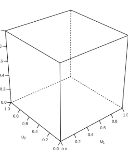
According to above definition shows thatCis a bivariate distribution function on the unit square[0,1]2whose margins are uniform on[0,1]. Both above definitions are connected by Sklar’s (1959) [42] via his theorem stated below, which now bears his name. In fact, the use of copulas allows solving the fundamental problem of determining the relationship between the joint distribution functions and their one-dimensional distributions by performing two basic tasks. First, find out one-dimensional margins (not necessarily from the same family) and secondly, choose a copula to link them. We now present Sklar’s theorem that justifies such a role. 0.0 0.2 0.4 0.6 0.8 1.0 0.0 0.2 0.4 0.6 0.8 1.0 0.0 0.2 0.4 0.6 0.8 1.0 u1 u2 pCopula

Fig. 2.1 surface plot of the independence copula

Theorem 2.1 (Sklar’s Theorem):

LetH be a joint distribution function with marginsF andG. Then there exists a copulaC

such that for all(x,y)∈ℜ¯ (extended real line),

H(x,y) =C(F(x),G(y)) (2.2)

IfF andGare continuous, thenCis unique; otherwise,Cis uniquely determined on(Range ofF)×(Range ofG). Conversely, ifCis a copula andF andGare distribution functions, then the functionH defined by (2.1) is a joint distribution function with marginsF andG. See proof in Nelsen (2006) [32]. The following corollary provides a means how to determine a copula function from the joint distribution and the generalized inverse of its marginals,F−1

(22)

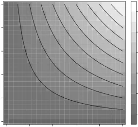
2.2 Definitions and properties 9 u1 u2 0.0 0.2 0.4 0.6 0.8 1.0 0.0 0.2 0.4 0.6 0.8 1.0 0.0 0.2 0.4 0.6 0.8 1.0

Fig. 2.2 contour plot of the independence copula

Corollary 2.1 (Sklar’s Theorem):

LetH,F,G,andCbe as defined above and letF−1andG−1be generalized inverses ofF and

G, respectively. Then for any(u,v)in[0,1]2

C(u,v) =H(F−1(u),G−1(v)) (2.3)

See proof in Nelsen (2006) [32].

Note that whenF and Gare continuous this result provides a method of constructing copulas from knowledge of joint and marginal distribution functions (see Section 2.5). Next, we describe some of the basic properties of copulas. Proofs of these properties can be found, for example, in Nelsen (2006) [32] and Cherubini et al. (2004) [6].

Property:1 The CopulaCis non-decreasing in each argument Theorem 2.2:

LetCbe a copula andu₁≤u₂foru₁,u₂∈[0,1]such that for allv∈[0,1]

C(u2,v)−C(u1,v)non decreasing on[0,1]

(23)

C(u,v2)−C(u,v1)non decreasing on[0,1]

Property:2 The CopulaCis uniformly continuous in its domain. Theorem 2.3:

LetCbe a copula and foru₁,u₂,v₁,v₂∈[0,1]such thatu₁≤u₂andv₁≤v₂then

|C(u2,v2)−C(u1,v1)| ≤ |u2−u1|+|v2−v1| (2.4)

Property:3. All partial derivatives of the copulaCexists.

Let C be a copula. For any v in [0,1], the partial derivative ∂C/∂uexists for almost all

u, and for such v and u, 0≤∂C(u,v)/∂u≤1. Similarly, For any u in [0,1], the partial

derivative∂C/∂vexists for almost allv, and for suchuand v, 0≤∂C(u,v)/∂v≤1. The

partial derivatives of the copula can be used to define conditional distribution functions by the relationships;

P[X ≤x|Y =y] =∂C(u,v)/∂vandP[Y ≤y|X=x] =∂C(u,v)/∂u (2.5)

whereu=F(x)andv=G(y)

Property:4. The CopulaCsatisfies the Frechet-Hoeffding bounds. Theorem 2.4:

LetCbe a copula. Then for every(u,v)in[0,1]2

W(u,v)≤C(u,v)≤M(u,v) (2.6)

whereW(u,v) =max(u+v−1,0)andM(u,v) =min(u,v)In the two dimensions, both the Frechet-Hoeffding lower bound,W, and upper bound,M, are copulas. However, at higher dimensions(d>2)the lower bound is never a copula; see for example Nelsen (2006) [32].

Definition 2.5:

The Product copula denoted byH is given by∏(u,v) =uv.

The product copula (∏), and the Frechet-Hoeffding boundsW and M are associated

with important statistical interpretations of random variables (see properties Property:5 and Property:6 below). A copula that includesH,W andM is called a comprehensive copula.

(24)

Property:5. Independence of random variables Theorem 2.4:

LetX andY be continuous random variables. Denote byCthe copula ofX andY . Then

X andY are independent if and only ifC=∏.

Property:6. Perfect dependence of random variables Theorem 2.5:

LetX andY be continuous random variables. Then the copula ofX andY isMif and only if each ofX andY is almost surely an increasing function of the other. Similarly, the copula ofX andY isW if and only if each ofX andY is almost surely a decreasing function of the other.

This theorem implies that the copulas M and W are associated with perfect positive de-pendence and perfect negative dede-pendence, respectively. One very attractive property of copulas is that they are invariant or change in a predictable way under strictly monotone transformations of random variables.

Property:7. Invariance property of Copulas Theorem 2.6 (Schweizer and Wolff, 1981 [40]):

LetX andY be continuous random variables with copulaC_XY. Then

1. If α and β are strictly increasing almost surely on Range of X and Range of Y ,

respectively, thenC_α_(X),β_(Y₎ =CXY ThusCXY is invariant under strictly increasing

transformations ofX andY

2. Ifα and β are strictly decreasing on almost surely on Range ofX and Range ofY,

then the copulasC₁,C₂ andC₃ of the pairs(α(X),Y),(X,β(Y)), and (α(X),β(Y))

respectively, are independent of the particular choices ofα andβ and are given by

C₁(u,v) =v−C_XY(1−u,v)

C₂(u,v) =u−C_XY(u,1−v)

C₃(u,v) =u+v−1+C_XY(1−u,1−v) See proof in Schweizer and Wolff (1981).

This interesting invariance property of copulas is very useful. Suppose we know the form of the copula for two variablesX andY but due to some practical reasons it is necessary to transform the data to log(x)and log(y). Then, because of the invariance property of copulas, the copula for the logarithm transformation log(x)and log(y)remains unchanged.

(25)

Property:8. The copula density exists everywhere in[0,1]2.

Definition 2.6:

The copula densityc(·,·)is defined asc(u,v) =∂2C(u,v)/∂u∂v.

Theorem 2.7:

The copula densitycexists almost everywhere in[0,1]2and is non negative.

Note that for continuous random variablesX andY, the copula densityccan be related to the density of the distribution functionsH denoted byhand the marginal distributionsF and

Gwith densities denoted by f andg, respectively. From the probability integral transforms we haveU =F(x) andV =G(Y) , as a result X =F−1(U) andY =G−1(V). Since for continuous random variables these transformations are strictly increasing and continuous we have c(u,v) =h(F−1(U),G−1(V))∗ ∂X/∂U ∂X/∂V ∂Y/∂U ∂Y/∂V ! (2.7) = h(F −1₍_U₎_,_G−1₍_V₎₎ f(F−1₍_U₎₎_g₍_G−1₍_V₎₎ It follows that, c(F(x),G(y)) = h(x,y) f(x)g(y) (2.8)

Thus, the joint density ofX andY is expressed as the product of the marginal and copula densities:

h(x,y) = f(x)g(y)c(F(x),G(y)) (2.9)

Next we state thed-dimensional(d>2)extension of Sklar’s theorem. Many properties of the d -dimensional copula can be analogously defined as in the two-dimensional case. Here we just give the d -dimensional extension of the Sklar’s theorem, further details can be found in Nelsen (2006) [32] and Cherubini et al. (2004) [6].

(26)

2.3 Some extended concepts of copulas 13

Theorem 2.8 (Sklar’s Theorem ind-dimensions ):

LetH be ad -dimensional distribution function with marginsF₁,F₂, ...,F_d. Then there exists ad-copulaCsuch that for all(x₁,x₂, ...,x_d)in ¯ℜd

H(x₁,x₂, ...,x_d) =C(F₁(x₁),F₂(x₂), ...,F_d(x_d)) (2.10)

IfF₁,F₂, ...,F_d are all continuous, thenCis unique; otherwise,Cis uniquely determined on RangeF₁× · · ·×RangeF_d . Conversely, ifCis ad -copula andF₁,F₂, ...,F_dare distribution functions, then the functionH defined by (2.3) is a d -dimensional distribution function with marginsF₁,F₂, ...,F_d

Corollary 2.2 (Sklar’s Theorem ind-dimensions):

LetH,C,F₁,F₂, ...,F_d, be as defined above and letF₁−1,F₂−1, ...,F_d−1be generalized inverses ofF₁,F₂, ...,F_d , respectively. Then for anyu₁,u₂, ...u_din[0,1]2

C(u₁,u₂, ...u_d) =H(F₁−1(u₁),F₂−1(u₂), ...,F_d−1(u_d)) (2.11)

2.3

Some extended concepts of copulas

In this section we summarize some important extended copula concepts, which have made remarkable contribution towards the growing interest in copula theory.

Survival Copula

For two random variablesX andY with marginal distributionsF andG, respectively and bivariate distribution functionH, the marginal survival functions ¯F and ¯Gand the bivariate survival function ¯Hare given by ¯F(x) =P(X >x),G¯(y) =P(Y >y)and ¯H(x,y) =P(X >

x,Y >y)respectively.

Definition 2.7:

The survival copula ˆC is a function, which relates the bivariate survival function to its marginal survival functions, i.e.,

¯

(27)

The survival copula ˆCis a copula, and is related to the copulaCofX andY via the equation ˆ

C(u,v) =u+v−1+C(1−u,1−v) (2.13)

Conditional or Time Dependent Copulas

In practice, in the presence of temporal dependence, which is a common feature of time series data, a powerful tool to specify the underlying models is conditional information with respect to past observations. Here we state the extended version of Sklar’s Theorem given in Patton (2006a) [35] and Fermanian and Scaillet (2005a [15]).

LetX,Y andW be continuous random variables withW be the conditioning variable. Let the joint distribution of (X,Y,W) be HXYW, denote the conditional distribution of(X,Y)

H_XY_|W(∞,y|w). Assume thatHXYW has all the required derivatives, and thatFX|W,GY|W,and H_XY_|W are continuous.

Definition 2.8 (Conditional copula , Patton (2006a) [35]):

G_Y_|W(·|w)is the conditional joint distribution function ofU=F_X_|W(X|w)andV=G_Y_|W(Y|w) givenW =w, where the variablesU andV are known as conditional probability integral transforms ofX andY givenW .

Patton (2006a) [35] has shown that the conditional copula function satisfies similar properties as that of the unconditional copula defined by Sklar (1959) [42]. Hence, the following version of Sklar’s theorem holds.

Sklar’s Theorem 2.9 (Conditional copula, Patton (2006a) [35]):

H_XY_|w=C(F_X|W(x|w),G_Y_|W(y|w)|w)for all (x,y)∈ℜ¯2and eachw∈ω¯. (2.4) Conversely,

(28)

function with conditional marginal distributionsF_X|W(·|w)andG_Y_|W(·|w).

Remark: This version of Sklar’s theorem for conditional distributions demands that the conditioning variable, W, must be same for both marginal distributions and the copula. Otherwise the functionHW may not be a joint conditional distribution function. Consider X|W₁,Y|W₂andC_XY_|w₁_,w₂ and specify

H_XY_|w₁_,w₂(x,y|w₁,w₂) =C F_X|W₁(x|w₁),G_Y_|W₂(y|w₂)|w₁,w₂ (2.14)

Then, H_XY_|w₁_,w₂(x,∞|w₁,w₂) =C F_X|W₁(x|w₁),1|w₁,w₂=F_X_|W₁(x|w₁)which is the con-ditional marginal distribution of X|W₁, which is the conditional marginal distribution of (X,Y)|W₁. Similarly,H_XY_|w₁_,w₂(∞,y|w1,w2) =C 1,GY|W2(y|w2)|w1,w2

=F_Y_|W₂(y|w₂)which is the conditional marginal distribution of Y|W₂, which is the conditional marginal dis-tribution of (X,Y)|W₂. Thus the function H_XY_|w₁_,w₂ cannot be the joint distribution of (X,Y)|(W₁,W₂). The only case H_XY_|W₁_,W₂ will be joint distribution of (X,Y)|(W₁,W₂) is whenF_X_|W₁(x|w₁) =F_X|w₁_,w₂(x|w₁,w₂) and F_Y_|W₁(y|w₁) =F_Y_|w₂_,w₂(y|w₁,w₂) that is when some conditioning variables affect the conditional distribution of one variable but not the other.

Remark.

Corollary 2.1 can be formulated in a manner that can help to extract the conditional copula from any bivariate conditional distribution. Fermanian and Scaillet (2005a) [15] provided the definition of conditional copula in terms of sigma fieldℑ.

Empirical Copula

Deheuvels (1979) [10] introduced empirical copulas. He called them empirical dependence functions.

Definition 2.9: Let (x_t,y_t), t =1,2, ...,n denote a sample of size n from a continuous bivariate distribution. The empirical copula functionC_nis given by

C_n t 1 n, t₂ n = 1 n n

∑

t=1 I(x_t ≤x_t₁,y_t ≤y_t₂) (2.15)

wherexti andyti, 1≤t1· ·· ≤ti≤nare order statistics from the sample andIis the usual

indi-cator function. Note that the sample versions of several measures of dependence/association can be expressed in terms of empirical copula analogous to the population versions of measures of dependence that can be expressed in terms of copulas.

(29)

2.4 Methods of Constructing Copulas 16

2.4

Methods of Constructing Copulas

First we note that there are several methods of constructing copulas, see for example Nelsen (2006) [32] and in this section we considered a few selected methods.

1. Inversion of Marginals: Let H he a two-dimensional distribution function with known continuous marginal distributions F andG and their inversesF−1 and G−1, respectively. Then we can find the unique copula as

C(u,v) =H(F−1(u),G−1(v)) (2.16)

Example:Gaussian Copula. Letφρ(x,y)be a standard bivariate normal distribution

function with coefficient of correlationρ and letφ(·)represents univariate standard

normal margin. Then, the Gaussian (Normal) copula is given by

C(u,v;ρ) =φρ φ−1(u),φ−1(v)

(2.17)

2. Method of Frailties:The concept of frailty has been extensively used in survival anal-ysis. Frailties can be used to construct various families of copulas (Oakes, 1989 [33]). Denote the frailty byZand assume that it is non negative with density f(z), distribution functionF(z), and Laplace transformLZ(t) =EZ(exp(−z)). Now, consider random

variablesX andY with survival functionsSX andSY respectively. LetBX andBY. be

two continuous baseline survival functions. Assume that the random variablesX andY

are conditionally independent given the frailtyZ. That is

and the joint survival functionS_XY(x,y)can be derived from

S_XY(x,y) = Z ∞

0

S_X(x|Z=z)S_Y(y|Z=z)f(z)dz (2.20)

Let us consider a special case where we assume that

(30)

such that the unconditional survival functions are given by,

S_X(x) =L_Z[−logB_X(x)] andS_Y(y) =L_Z[−logB_Y(y)] (2.22)

It follows that, SXY(x,y) = Z ∞ 0 SX(x|Z=z)SY(y|Z=z)f(z)dz =R∞ 0 [BX(x)]z[BY(y)]zf(z)dz =E_Z{B_X(x)B_Y(y)z}

=E_Z{exp(z[logB_X(x) +logB_Y(y)])}

=L_Z[−(logB_X(x) +logB_Y(y))] Further we have,

−log(B_X(x)) =L_Z−1(S_X(x)) and −log(B_Y(y)) =L_Z−1(S_Y(y)) (2.23)

Thus, we can write the joint survival function is given by,

(S_XY(x,y) =L_ZL−_Z1(S_X(x)) +L−_Z1(S_Y(y)) (2.24) Finally, it follows that the copula is given by

C(u,v) =L_ZL_Z−1(u) +L−_Z1(v) (2.25) whereu=SX(x)andv=SY(y)

Example: Gumbel-Hougaard Copula. Suppose the frailty Z has a positive stable distribution with Laplace transform given by

L_Z(t) =exp(−t1/δ)

Hence, using (2.8) we have the Gumbel-Hougaard family of copulas given by

C(u,v) =exp

−h(−log(u))δ_{+ (}₋

log(v))δi1/δ

Remark: The advantage of the frailty concept is that it allows us to interpret the dependence of the random variables in such away that a frailty that contributes to the dependence of the random variables may exist.These class of copulas generated by frailty models are a subclass of the Archimedean copulas defined on a more general functions called "Generators" discussed below.

(31)

3. Method of Generators: Another important way of constructing copulas is using a functionφ called a "Generator" that satisfies the following properties

(a) φ :[0,1]→[0,∞]

(b) φ is continuous and strictly decreasing function,

(c) φ is such thatφ(1) =0

The pseudo inverse ofφ is the functionφ[−1][0,∞]→[0,1]given by,

φ[−1](t) = (

φ−1(t) 0≤t≤φ(0)

0 φ(0)≤t≤∞

Ifφ(0) =∞, then the pseudo inverseφ[−1]=φ−1, inverse ofφ.

Theorem 2.10: Let the Generatorφ be as defined above and letφ[−1]be the pseudo

inverse ofφ. Then, the functionCfrom[0,1]2→[0,1]given by

C(u,v) =φ[−1](φ(u) +φ(v)) (2.26)

is a copula if and only ifφ is convex. Copulas of the form (2.9) are called Archimedean

copulas. Some examples and properties are discussed in subsequent sections; see details in Nelsen (2006) [32], Chapter 4).

Example:(Frank Copula ) Suppose the generator is given by

φ(t) =−log

1−e−δt

1−e−δ

and inverseφ−1(u) =−_δ1log h

1−1−e−δ

e−u

i

Thus, the resulting copula is the Frank’s family given by

C(u,v) =−1 δ log  1− 1−e−δu 1−e−δv 1−e−δ  

4. Polynomial Approximations to copulasPolynomials are used in the approximation of distribution functions. To this end, Hoeffding (1940) [48] used Legendre polyno-mials to approximate bivariate "standard distributions" later called copulas. Recently, Sancetta and Satchell 2004 [37]) introduced Bernstein copula defined by Bernstein polynomials that are closed under differentiation.

(32)

2.5 Important families of copulas 19

Definition 2.10 (Bernstein copula, Sancetta and Satchell (2004) [37]): Let α k1 m1, k2 m2

valued constant, k∈ {1,2} such that 1≤k ≤mi,i =1,2 and the

Bernstein polynomials given by

P_k_i_,m_i(u_i) = m_i ki u_ik_i(1−u_i)k_i If C_B:[0,1]2→[0,1] (2.27) where C_B(u₁,u₂) = m1

∑

k1=1 m2

∑

k2=1 α k₁ m1 , k2 m2 P_k₁_,m₁(u₁)P_k₂_,m₂(u₂) (2.28)

satisfies the properties of the copula function in Definition (2.4), thenC_B is called the Bernstein copula. Some statistical properties of Bernstein copula are studied by Sancetta and Satchell (2004) [37]. In particular, they have shown that the coefficients of the Bernstein copulaC_B have a direct interpretation as the points of some arbitrary approximated copula,C, i.e.,

α k₁ m₁, k₂ m₂ =C k₁ m₁, k₂ m₂ (2.29)

2.5

Important families of copulas

In the copula literature several examples of copula functions are introduced. Most of the copulas belong to members of families with one or more real valued parameters. In this section we present a very brief overview of some parametric families of copulas. Extensive surveys of families of copulas can be found in Joe (1997) [22] and Nelsen (2006) [32].

2.5.1

Farlie-Gumbel-Morgenstern’s (FGM) Family

The FGM family is a symmetric and one parameter family of copulas whose functional form is a polynomial inuand inv. That is, forδ ∈[−1,1]then the function is given by

C_δ(u,v) =uv+δuv(1−u)(1−v) (2.30)

(33)

2.5.2

Archimedean Copulas

The Archimedean copulas are given by the general expression

C(u,v) =φ[−1](φ(u) +φ(v)) (2.31)

whereφ is a "Generator" defined in Section 2.5 above.

The Archimedean copulas have a wide range of applications as indicated in Nelsen (2006) [32] because of the ease with which they can be constructed, the many parametric families of copulas belonging to this class, the great variety of dependence structures offered by this class and the nice properties possessed by the members of this class such as extension to higher dimensions, convenient in developing criteria for copula model selection and establishing relationship with nonparametric measures of associations, etc. Genest and MacKay (1986a,b) [19] have presented many properties of this class of copulas, which made them extremely suitable for statistical applications. Next, we present brief descriptions to four members of Archimedean family of copulas that are used in the subsequent chapters.

1. Gumbel’s Family.

The Gumbel copula is given by

C(u,v;δ) =exp −(u˜δ+v˜δ) 1 δ (2.32)

where ˜u=−log(u),v˜=−log(v) with copula density,

c(u,v;δ) =C(u,v;δ)[uv]−1 (u˜v˜) δ−1 (u˜δ₊_v_˜δ₎2− 1 δ (u˜δ₊_v_˜δ₎ 1 δ ₊ δ−1 (2.33)

This family has properties like upper tail dependence, product copula forδ=1,

Frechet-Hoeffding upper bound copula forδ →∞(see Joe, 1997, Family B6, p. 142). These

properties are the subject of the next section.

2. Clayton’s (or Kimeldrof and Sampson’s) Family.

This copula is referred as Clayton’s copula, for example, in Nelsen (2006) [32] and Kimeldrof and Sampson’s copula in Joe (1997) [22]. This copula is given by

C(u,v;δ) = (u˜δ+v˜δ)−1)

−1

δ

(34)

with copula density,

c(u,v;δ) = (1+δ)[uv]−δ−1(u˜δ+v˜δ)−2−

1

δ _(2.35)

This family has properties like lower tail dependence, product copula for δ →0,

Frechet Hoeffding upper bound copula forδ →∞(see Joe, 1997 [22], Family B4, p.

141). 0.0 0.4 0.8 0.0 0.4 0.8 δ = −0.95 u1 u2 0.0 0.4 0.8 0.0 0.4 0.8 δ = −0.75 u1 u2 0.0 0.4 0.8 0.0 0.4 0.8 δ = −0.25 u1 u2 0.0 0.4 0.8 0.0 0.4 0.8 δ = −0.1 u1 u2 0.0 0.4 0.8 0.0 0.4 0.8 δ = 0.1 u1 u2 0.0 0.4 0.8 0.0 0.4 0.8 δ = 1 u1 u2 0.0 0.4 0.8 0.0 0.4 0.8 δ = 5 u1 u2 0.0 0.4 0.8 0.0 0.4 0.8 δ = 15 u1 u2 0.0 0.4 0.8 0.0 0.4 0.8 δ = 200 u1 u2

(35)

3. Frank’s Family.

The Frank copula is given by

C(u,v;δ) =−δ−1log   h (1−e−δ)−(1−e−δu)(1−e−δv) i (1−e−δ)   (2.36)

c(u,v;δ) = h δ(1−e−δ)e−δ(u+v) i (1−e−δ)−(1−e−δu)(1−e−δv)2 (2.37)

This family has properties like reflection symmetry, product copula forδ →0, Frechet

Hoeffding lower and upper bound copulas forδ → −∞andδ →∞, respectively (see

Joe, 1997 [22], Family B3, p. 141). 4. Joe’s Family

The Joe’s copula is given by

C(u,v;δ) =1−

¯

uδ₊_v_¯δ₋_u_¯δ_v_¯δ1/δ

δ ≥1 (2.38)

c(u,v;δ) = ¯ uδ+v¯δ−u¯δv¯δ −2+1/δ ¯ uδ−1v¯δ−1 δ−1+u¯δ+v¯δ−u¯δv¯δ (2.39) where ¯u=1−uand ¯v=1−vThis family has properties like upper tail dependence, product copula forδ =1, Frechet Hoeffding upper bound copula forδ →∞(see Joe,

1997 [22],Family B5, pp. 141-142).

2.5.3

Elliptical Copulas

Elliptical copulas are copulas associated with elliptical distributions. For definitions of elliptical distributions see for example Embrechts et al. (2002) [14]. The Gaussian copula and the t-copula are examples of elliptical copulas. For example, the Gaussian copula is given by

(36)

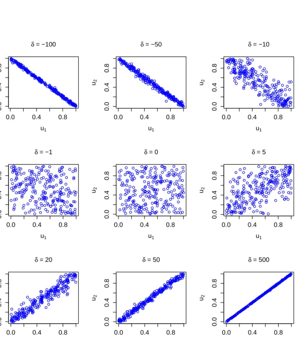
2.5 Important families of copulas 23 0.0 0.4 0.8 0.0 0.4 0.8 δ = −100 u1 u2 0.0 0.4 0.8 0.0 0.4 0.8 δ = −50 u1 u2 0.0 0.4 0.8 0.0 0.4 0.8 δ = −10 u1 u2 0.0 0.4 0.8 0.0 0.4 0.8 δ = −1 u1 u2 0.0 0.4 0.8 0.0 0.4 0.8 δ = 0 u1 u2 0.0 0.4 0.8 0.0 0.4 0.8 δ = 5 u1 u2 0.0 0.4 0.8 0.0 0.4 0.8 δ = 20 u1 u2 0.0 0.4 0.8 0.0 0.4 0.8 δ = 50 u1 u2 0.0 0.4 0.8 0.0 0.4 0.8 δ = 500 u1 u2

(37)

2.5 Important families of copulas 24 0.0 0.4 0.8 0.0 0.2 0.4 0.6 0.8 1.0 δ = 1 u1 u2 0.0 0.4 0.8 0.0 0.2 0.4 0.6 0.8 1.0 δ = 1.5 u1 u2 0.0 0.4 0.8 0.0 0.2 0.4 0.6 0.8 1.0 δ = 2 u1 u2 0.0 0.4 0.8 0.0 0.2 0.4 0.6 0.8 1.0 δ = 6 u1 u2 0.0 0.4 0.8 0.0 0.2 0.4 0.6 0.8 1.0 δ = 10 u1 u2 0.0 0.4 0.8 0.0 0.2 0.4 0.6 0.8 1.0 δ = 50 u1 u2

(38)

2.6 Dependence Measures 25

c(u,v;δ) = 1 (1−δ2) e −1 2(1−δ2)(X 2_+Y2₋₂_δXY₎ n e12(X2+Y2) o (2.41)

whereX =φ−1(u)andY =φ−1(v)We note that multi-parametric families of copulas are

extensively discussed in Joe (1997) [22]. Here we give one example from two parametric families of copulas.

2.5.4

Frechet’s Family

The Frechet’s family is a two-parameter family of copulas given as a convex linear combina-tion of the copulasπ,W andM, i.e.,

C_{α β}(u,v) =αM(u,v) + (1−α−β)π(u,v) +βW(u,v) (2.42)

whereα,β ∈[0,1]withα+β ≤1

2.6

Dependence Measures

In this section we deal with different ways in which copulas can be used in the study of dependence between random variables. There are a variety of ways to describe and measure the dependence or association between random variables. The multivariate normal distribution and linear correlation have been the basis for most dependence modeling in practice. In fact, linear correlation is a good measure of dependence in the context of multivariate normal distributions or elliptical distributions in general but it has several problems if applied to distributions other than elliptical distributions (Embrechts et al, 2002 [14]). Alternative measures of dependence using nonparametric methods are also common in practice. Copulas are capable of describing these measures of dependence and also capturing any form of dependence structure. Many measures of dependence have been introduced and studied in the literature. Among them the most widely used measures are: the Pearson’s coefficient of correlation(r), Spearman’s rho(ρs)introduced by

Spearman(1904) [46], and Kendall’s tau(τ)introduced by kendall (1938) [25]. Definitions

of these measures and their relation to copulas can be found, for example, in Nelsen (2006) [32] and Joe (1997) [22]. Let X and Y be two random variables and letF,G,H,andC be defined as in Section 2.2.

(39)

Pearson correlation coefficient

r(x,y) = 1 σ(x)σ(y) Z ∞ −∞ Z ∞ −∞ [H(x,y)−F(x)G(y)]dxdy (2.43)

whereσ(·)represent for standard deviation.

Spearman’s rho ρ(x,y) =12 Z ∞ −∞ Z ∞ −∞ [H(x,y)−F(x)G(y)]dF(x)dG(y) (2.44) Kendall’s tau τ(x,y) =4 Z ∞ −∞ Z ∞ −∞ H(x,y)dH(x,y) −1 (2.45)

Moreover, Schweizer and Wolff (1981) studied the following three nonparametric measures of associationσSW,γ andKbased onL1,L2andL∞distances, respectively. These measures are given by,

1. σSW(X,Y) = Z ∞ −∞ Z ∞ −∞ |H(x,y)−F(x)G(y)|dF(x)dG(y) 2. γ(X,Y) = 90 Z ∞ −∞ Z ∞ −∞ [H(x,y)−F(x)G(y)]2dF(x)dG(y) 1₂ 3. κ(X,Y) =4 sup x,y∈R |H(x,y)−F(x)G(y)|

Now, it is important to note that these measures of dependence can be expressed in terms of copulas (see Schweizer and Wolff, 1981 [40]). LetU =F(X)andV =G(Y)be probability integral transformations. Using Sklar’s framework[H(x,y) =C(F(X),G(y))]we have

• r(X,Y) = 1 σ(X)σ(Y) Z 1 0 Z 1 0 [C(u,v)−uv]dF−1(u)dG−1(v) • ρ(X,Y) =12 Z 1 0 Z 1 0 [C(u,v)−uv]dudv • τ(X,Y) =4 Z 1 0 Z 1 0 C(u,v)dC(u,v)−1 • σSW(X,Y) = Z 1 0 Z 1 0 |C(u,v)−uv|dudv • γ(X,Y) = 90 Z 1 0 Z 1 0 [C(u,v)−uv]2dudv 1₂

(40)

• κ(X,Y) =4 sup

x,y∈R

|C(u,v)−uv|

Remark:Using the copula transformations at least two things are apparent. First, integrals over the plane are transformed into integrals in the unit square. Second, the nonparametric measures,ρS,τ,σSW,γ andκ, distinguished from the coefficient of correlation,r, in that they

are functions of the copula alone, i.e., it is only the coefficient of correlation that depends on the marginals but all others are scale free measures.

Furthermore, in the study of properties of Archimedean copulas, Genest and Mac Kay (1986b [19]) provided a simplified version of Kendall’s tau, which is stated in the following theorem.

Theorem 2.11 (Kendall’s Tau for Archimedean Copulas, Genest and MacKay (1986b) [19]):

Let X andY be random variables with an Archimedean copulaChaving generator φ.The

population version of Kendall’s tau ,r, for the random variablesX andY is given by

τ=1+4

Z 1

0

φ(t)

φ′(t)dt (2.46)

whereφ′is the first derivative ofφ. See Genest and MacKay (1986b) [19] for proof.

Example: Consider the Clayton copula with generatorφ(t) = t

−δ₋₁

δ for δ >0. Then,

Kendall’s tau for this copula is

τ=1+4 Z 1 0 tδ₊₁ δ dt = δ δ+2 (2.47)

2.6.1

Measure of concordance

Definition: (Nelsen (2006) [32], page 136) A numeric measure of association between two continuous random variablesX andY whose copula isCis a measure of concordance if it satisfies the following properties:

1. κ is defined for every pairX,Y of continuous random variables;

2. −1=κX,−X ≤κC≤κX,X =1;

3. κX,Y =κY,X

4. ifX andY are independent, thenκX,Y =κC⊥ =0;

(41)

6. ifC1≺C2thenκC1 ≤κC2;

7. if{(X_n,Y_n)}is a sequence of continuous random variables with copulasC_n, and if{C_n}

converges point wise toC, then lim

n→∞κCn =κC

Among all the measures of concordance, three famous measures play an important role in non-parametric statistics: the Kendall’s tau, the Spearman’s rho and the Gini indice. They could all be written with copulas, and we have (Schweitzer and Wolff [1981] [40]) Nelsen [1998] [31] presents some relationships between the measuresτ andρ , that can be

summarized by a bounding region. In Figure 2.6 , we have plotted the links betweenτ andρ

for normal copulas. We note that the relationships are similar. However, some copulas do not cover the entire range[−1,1]of the possible values for concordance measures. For example, Kimeldorf-Sampson, Gumbel, Galambos and Hausler-Reiss copulas do not allow negative dependence. −1.0 −0.5 0.0 0.5 1.0 −1.0 −0.5 0.0 0.5 1.0

Correlation parameter of normal copula ρs and τ Diagonal ρs τ

(42)

2.6.2

Measure of dependence

Definition 2.10:(Nelsen (1998) [31] A numeric measure of association between two contin-uous random variablesX andY whose copula isCis a measure of dependence if it satisfies the following properties:

1. δ is defined for every pairX,Y of continuous random variables;

2. 0=δ_C⊥ ≤δC≤δC+=1

3. δX,Y =δY,X

4. δX,Y =δC⊥=0 if and only ifX andY are independent;

5. δX,Y =δC+ =1 if and only if each of X andY almost surely a strictly monotone

function of the other;

6. ifh₁andh₂are almost surely strictly monotone functions onIm(X)andIm(Y) respec-tively, then

δ_h₁_(x),h₂_(y)=δX,Y

7. if{(X_n,Y_n)}is a sequence of continuous random variables with copulasC_n, and if{C_n}

converges point wise toC, then lim

n→∞δCn =δC

2.6.3

Tail Dependence

Tail dependence measure refers to the dependence that arises between random variables from extreme observations. Upper tail dependence exists when large extreme values occur jointly, while lower tail dependence exists when small extreme values occur jointly. Another important feature of copulas is that the upper and lower tail dependence measures can be expressed in terms of copulas.

Definition 2.11: (Upper tail dependence):

LetX andY be two continuous random variables with marginal distribution functionsF

andG, and copulaC. Then the coefficient of upper tail dependence ofX andY is:

λu= lim u→1−Pr

X>F−1(u)|Y >G−1(u) (2.48) provided that a limitλu∈(0,1]exists. Ifλu∈(0,1],XandY are said to be asymptotically

(43)

in the upper tail. Using the probability integral transformsU =F(X) andV =G(Y) the coefficient of upper tail dependence can be rewritten as

λu= lim u→1−

Pr[U >u|V >v] (2.49)

Further, this can be expressed in terms of copulas as follows:

λu= lim u→1−

1−2u−C(u,u)

1−u (2.50)

Definition 2.12: (Lower tail dependence):

LetX andY be two continuous random variables with marginal distribution functionsF and

G, and copulaC. Then the coefficient of lower tail dependence ofX andY is:

λL= lim u→0+Pr

X ≤F−1(u)|Y ≤G−1(u)= lim

u→0+Pr[U≤u|V ≤v] (2.51)

provided that a limitλL∈(0,1]exists. IfλL∈(0,1],X andY are said to be asymptotically

dependent in the lower tail; ifλL=0,X andY are said to be asymptotically independent in

the lower tail.This can be expressed using copulas as

λL= lim u→0+

C(u,u)

u (2.52)

Independence

The most commonly used dependence property is the assumption that there is no dependence that is the random variables are independent. If two continuous random variables are independent, then their copula is the product copula,n, see Section (2.2) property 5. Perfect Dependence

We have seen in Section (2.2) property 6 that one function is almost surely a monotone function of the other (perfect dependence) whenever the copula is eitherW or M . We note that other dependence forms that lie between the extremes independence and perfect dependence and their relationship with copulas are discussed in Joe (1997) [22] and Nelsen (2006) [32].

(44)

Chapter 3

Statistical inference of copulas

3.1

Estimation and Asymptotic Properties

In this section we present various methods related to estimation of copulas. Consider a correctly specified copula that belongs to a parametric familyC={C(·,δ),δ ∈ℜ}.

Consis-tent and asymptotically normally distributed estimates can be obtained through maximum likelihood methods (one-stage or two-stages) mainly using a fully parametric or a semi-parametric approach, see for details in Joe (1997) [22], Genest et al. (1995) [18] and Shih and Louis (1995) [41]. Alternatively, one can estimate copulas by nonparametric methods using empirical copula (Deheuvels, 1979) [10]. Recently, for multivariate time series models Patton (2006a, b) [35] [34] employed two-stage maximum likelihood estimation for con-ditional copulas. Similarly, Chen and Fan (2006) [4] have studied the two-stage approach for a Markov time series under the semiparametric setup. We now give a survey of various approaches of estimation suggested in the literature for the i.i.d. multivariate setup. Consider a random sample of d variables and n number of observations represented by the vector

x= (x1t,x2t, ...xdt),t=l, ...,n. Consider a copula-based model for the random vectorX ,

with distribution function

H(x₁,x₂...x_d;θ1, ....θd,δ) =C(F1(x1,θ1), ...Fd(xd,θd);δ) (3.1)

whereθi,i=l, ...,d,each being scalar or vector of parameter(s) of the marginal distributions Fi,i=1,2, ...,dandδ is a scalar or vector of the copula parameter(s). Letη = (θ1, ...θd,δ)

(45)

3.1 Estimation and Asymptotic Properties 32

3.1.1

Maximum likelihood Estimation (MLE)

Consider the log-likelihood function based on (2.2), that is given by :

l(η;x) = n

∑

j=1 d

∑

i=1 logfi(xit;θi) + n

∑

i=1 logc(F1(x1i,θ1), ...Fd(xdi,θd);δ) (3.2)

Thus, the maximum likelihood estimator ˆη of the parameter vectorη is the solution of

∂l(η,x)

∂ η =0

Letη0be the true value ofη. Under standard regularity conditions, consistency and

asymp-totic normality properties of the estimator ˆη have been established; see, for example, Joe

(1997) [22]. That is,

√

n(−η0)→N(0,I−1)in distribution,

whereIis the Fisher Information matrix.

The estimation of Maximum likelihood Estimation (MLE) can be carried out by using R program’s codes which is include in Appendix section,then that corresponding out put given below.

> summary(mle)

Call: fitMvdc(data = X, mvdc = mcc, start = start) Maximum Likelihood estimation based on 2000

2-dimensional observations. Copula: claytonCopula Margin 1 : Estimate Std. Error m1.mean 0.004963 0.018 m1.sd 0.990165 0.007 Margin 2 : Estimate Std. Error m2.rate 0.9853 0.021 Clayton copula, dim. d = 2

Estimate Std. Error alpha 4.99 0.124

The maximized loglikelihood is -2923 Optimization converged

(46)

3.1 Estimation and Asymptotic Properties 33 function gradient

78 16

Note that as the number of parameters increases computational problems may arise when using MLE method. An alternative approach that helps to reduce computational problem is the use of two-stage method discussed below.

3.1.2

Inference Functions for Margins (IFM ) method

For copula-based models this method is first followed by Joe and Xu (1996) [24], in order to exploit the fundamental idea of copula theory that allow the separation of the univariate margins from the dependence structure or copula. This method consists of estimating the model parameter by finding solutions for conveniently defined set of inference (estimating) functions. In this method the score functions of the margins and the copula constitute the set of inference functions. Thus, according to the two-stage estimation method, the parameters of the marginal distributions are estimated separately from the parameters of the copula. In other words, the estimation process is divided into two steps:

Step 1.

Estimating the parameters θi,i=1,2, ...d, using maximum likelihood method from the

respective marginal log-likelihoods, i.e., consider the marginal log-likelihoods

l_i(θi;xi) = n

∑

j=1

logf_i(x_{i j};θi) (3.3)

Then, the maximum likelihood estimator ˜θiof the parameter vectorθiis the solution of

Thus, we have the estimates ˜θ1, ...θ˜d for the marginal parameters

Step 2.

To Estimate the vector of copula parameters δ, first substitute the marginal estimates

˜

θ1, ...θ˜d to the copula log-likelihood l_c(δ;x,θ˜1, ...θ˜d) = n

∑

t=1 logc F₁(x₁_t; ˜θ1), ...Fd(xdt; ˜θd);δ (3.4)

Then, the pseudo maximum likelihood estimator S of the parameter vector ˜δ is the solution

to

∂lc δ;x,θ¯1, ...θ¯d

(47)

Therefore, the estimator ¯η=

˜

θ1, ...θ˜d,δ˜

is referred as the two-stage maximum likelihood estimator ofη= (θ1, ...θd,δ). Joe and Xu (1996) [24] established asymptotic normality

of this estimator. Let the inference functions be denote by the vectorg(x,η):

The estimation of Inference Functions for Margins (IFM ) can be carried out by using R program’s codes which is include in Appendix section,then that corresponding out put given below.

> summary(ifme)

Call: fitCopula(copula, data = data, method = "ml")

Fit based on "maximum likelihood" and 2000 2-dimensional observations. Clayton copula, dim. d = 2

Estimate Std. Error alpha 4.932 0.116

The maximized loglikelihood is 1886 Optimization converged

Number of loglikelihood evaluations: function gradient

4 4

3.1.3

Canonical Maximum Likelihood (CML) method

Both the MLE and IFM methods are based on some specified parametric form of the univariate margins. The choice of the best possible fit distributions for the margins is of course crucial. Hence, to avoid the risk involved in choosing parametric marginal models and without much information loss on the dependence structure, one can consider non-parametric marginal models. The semi parametric copula-based model estimation procedure also involves two steps:

Step 1.

Transform the observed data vectorx_t= (x₁_t, , , ...,x_dt), t=1,2, ...,ninto uniform values called pseudo-observations using rescaled empirical distributions defined by

F_in(x) =1 n n

∑

t=1 [X_it ≤x] for i=1,2, ...d (3.6)

where 1[·] represents indicator function. Let the transformed observation be denoted by (u˜₁, ....,u˜_dt) = (F₁_n(x₁_t), ...,F_dn(x_dt))fort=1, ...n.

(48)

To Estimate the vector of copula parametersδ, first substitute the transformed observations

(u˜1, ....,u˜dt)into the copula log-likelihood

l_c(δ; ˜u1, ....,u˜dt) = n

∑

t=1

logc(u˜₁, ....,u˜_dt;δ) (3.7)

Step 3.Then, the pseudo maximum likelihood estimator ˜δ of the parameter vectorδ is

the solution to

∂lc

∂ δ =0 (3.8)

Genest et al. (1995) established consistency and asymptotic normality of the semi-parametric estimator ˜δn.

The estimation of the Canonical Maximum Likelihood (CML) can be carried out by using R program’s codes which is include