Kernel Conditional Quantile Estimation via Reduction Revisited
Novi Quadrianto∗, Kristian Kersting†, Mark D. Reid∗, Tib´erio S. Caetano∗ and Wray L. Buntine∗ ∗SML, NICTA & RSISE, ANU
Canberra ACT, Australia
Email:{firstname.lastname}@nicta.com.au †Fraunhofer IAIS
Sankt Augustin, Germany
Email:{firstname.lastname}@iais.fraunhofer.de
Abstract—Quantile regression refers to the process of es-timating the quantiles of a conditional distribution and has many important applications within econometrics and data mining, among other domains. In this paper, we show how to estimate these conditional quantile functions within a Bayes risk minimization framework using a Gaussian process prior. The resulting non-parametric probabilistic model is easy to implement and allows non-crossing quantile functions to be enforced. Moreover, it can directly be used in combination with tools and extensions of standard Gaussian Processes such as principled hyperparameter estimation, sparsification, and quantile regression with input-dependent noise rates. No existing approach enjoys all of these desirable properties. Experiments on benchmark datasets show that our method is competitive with state-of-the-art approaches.
Keywords-Regression; Quantile Regression; Gaussian Pro-cesses;
I. INTRODUCTION
In most regression studies, we are typically interested in inferring a real-valued function whose values correspond to the mean of response variables conditioned on the ex-planatory variables. The application of this conditional mean regression is ubiquitous. There are, however, many important applications where we are interested in estimating either the median or other quantiles such as estimating the potential amount of money a customer can spend on a product rather than his/her expected spending [1]. This is called quantile regression and was introduced by Koenker and Bassett [2]. The unobservable nature of quantiles means that their pre-diction is a challenging task. If we had a modelp(y|x)of the conditional distribution of response variables y conditioned on the explanatory variables x, however, their prediction would be much simpler as quantile estimation essentially involves slicing this distribution at a certain quantile level. This slicing operation is a convex optimization problem. Al-though we arereducinga hard quantile estimation problem to yet another hard problem, i.e. distribution modeling, the latter is a well-studied subject in machine learning in particu-lar Gaussian processes. At first glance, the usage of Gaussian process distribution modeling for learning problems such as classification or regression might violate Vapnik’s paradigm of estimating only the relevant parameters directly [3].
This paradigm is in favor of estimating latent functions while sidestepping distribution modeling. However, there have been several studies that show superiority of Gaussian processes based methods to infer flexible latent functions [4], [5]. Our reduction approach is similar in spirit to the Langford’s et al. [6] method in reducing quantile estimation problem to series of classification problems.
Therefore, we propose in this paper to estimate condi-tional quantile functions within a Gaussian process model [7]. The well-known advantage of using such type of model over non-Bayesian models is that of having an explicit probabilistic formulation. This allows us to have a principled way of performing model selection, as well as a predictive posterior probability distribution over response variables. In terms of quantile estimation, the latter is particularly useful when we have censored or missing response variables [8]. From a practical point of view, our estimator can be easily sparsified, therefore being able to handle large datasets, and can take input dependent noise into account. More importantly, our derived quantile estimator has the desirable property that the estimated conditional functions at different quantiles can never cross or overlap each other. Quantile crossing occurs because each conditional quantile function is independently estimated, and it has traditionally been one of the challenging problems in the field [8], [9]. To our knowledge, our quantile estimator is the first that enjoys both sparsifiable and non-crossing properties while being competitive with state-of-the-art alternatives as we will show in our experiments.
Our contributions:
− A quantile estimator within a Bayes risk minimization framework using a Gaussian process prior.
− A specific example of Bayes quantile estimator which enjoys non-parametric, probabilistic model, principled learning of free parameters, sparse approximation, het-eroscedasticity and enforced non-crossing constraint. − A novel Gaussian processes treatment of
input-dependent noise which allows jointly learning the free parameters of the latent and observed processes. − A theoretical analysis of our proposed estimator in
II. RELATEDWORK
Most of existing work focuses on estimating each condi-tional quantile function separately. A standard technique for conditional quantile estimation is based on a linear model [2]. In this model, the τ-th conditional quantile function of y given x is assumed to be a linear function of the vector of regressors, i.e. qτ(x) := hx, β(τ)i, where β(τ) is a vector of coefficients dependent on τ. Estimation of coefficients is done by minimizing the pinball loss function. It is shown that the minimization can be reformulated as a linear programming problem and can be solved efficiently with interior point techniques [8].
The assumption of a linear relationship between the re-gressors and the conditional quantile function is quite restric-tive. Takeuchi et al. [10] propose a nonparametric approach to quantile regression based on kernel methods. The dual of a regularized version of pinball loss minimization is solved via standard quadratic programming techniques. Several extensions to incorporate commonly desired constraints such as non-crossing constraints and a monotonicity constraint are also discussed. This method provides state-of-the-art performance.
Langford et al. [6] show that the quantile regression problem can be reduced to a series of classification problems such that a small average error rate on the classification prob-lems leads to a provably accurate estimate of the conditional quantile. The estimation ofτ-th conditional quantile function is first reduced to a set of importance weighted binary classification problems. This problem is further reduced to ubiquitous unweighted binary classification problem via rejection sampling. This method is computationally efficient thus is able to handle large datasets.
The closest work to Quantile Gaussian processes is the work of Yu and Moyeed [11]. They introduce a Bayesian approach for quantile estimation based on the linear model. An asymmetric Laplace distribution is used as a likelihood function, p(y|x, β(τ)), and the prior on the coefficients is chosen to be improper uniform, (p(β(τ)) ∝ 1). Although the prior is improper, they proved that the posterior dis-tribution will be proper. A Markov chain Monte Carlo (MCMC) method is used to infer this posterior distribution,
p(β(τ)|x, y). Finally, the posterior mean is used for quantile estimation, i.e. qτ(x) := hx, βMAP(τ)i. We focus on a
different notion of prior distribution, usage of any likelihood function, and a different procedure for quantile estimation. Precisely these differences allow us to derive the desirable properties mentioned in the introduction.
III. QUANTILEESTIMATION AS ANOPTIMIZATION PROBLEM
Givenm observed data points D={(xi, yi)}mi=1, where yi ∈ Y (the set of outputs) and xi ∈ X (the set of regressors or inputs), the goal of quantile regression is to
L
τ(
ξ
)
τ
−
1
τ
ξ
0
0
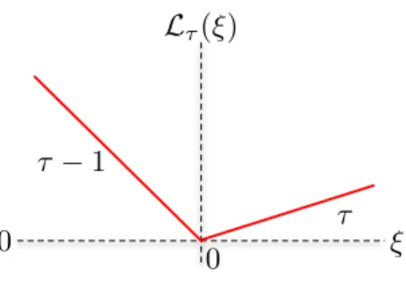
Figure 1. The pinball loss function.
infer a conditional quantile function qτ(x) from observed data points.
Definition 1 (Conditional Quantile): Letτ ∈(0,1). The conditional quantile qτ(x) for a pair of random variables (x, y) ∈ X ×R is defined as the function qτ : X → R for which pointwiseqτ(x)is the infimum overq for which Pr(y≤qτ|x) =τ.
The idea behind quantile regression arises from the ob-servation that minimizing the `1-loss function yields the median. The symmetry of the`1-loss function implies that minimization ofPm
i=1|yi−q| must give an equal number of yi−q terms lying on either side of zero. Koenker and Bassett [2] generalize this idea to obtain a quantile regression estimator by tilting the loss function. This loss function is given in Figure 1 and is known as a pinball loss function,
Lτ(ξ) :=n τ ξ, ifξ≥0 (τ−1)ξ, ifξ <0.
In this paper, our goal is to estimate the latent quantile function qτ(x) in a Bayesian framework with a Gaussian Process prior, which we will develop in the next section.
IV. BAYESIANFRAMEWORK
Assuming we can estimate the conditional distribution
p(y|x), the Bayes quantile estimator is found by minimizing expected value of the pinball loss function, i.e.
q(τopt)= argmin qτ Z Lτ(y−qτ)p(y|x)dy= argmin qτ Rτ(qτ) (1) whereRτ(qτ) :=Ep(y|x)[Lτ(y−qτ)]is the Bayes risk.
Lemma 2: The Bayes risk in Equation (1) is convex in
qτ.
Proof: The Bayes risk is a convex combination of convex loss functions, which must itself be convex.
The subsequent sections will deal with modeling the conditional distribution p(y|x). We will describe a model based on Gaussian processes framework. Before introducing the model, let us briefly review Gaussian processes.
Gaussian Process Prior: In the Gaussian process framework, the output yi at input location xi is assumed to be a corrupted version of a latent function q(xi), i.e.
process can be used to define a prior distribution over these latent functions [7],q∼ GP(m(x), k(x, x0)),wherem(x)is the mean function (assumed to be zero) and the covariance
k(x, x0) between functions at input xandx0 is defined by Mercer kernel functions [7].
Likelihood for Quantile Regression: In the Bayesian setting, there is a distinction between the likelihood function and the loss function. The likelihood defines the probability of observing the noisy outputs given the latent functions, whereas the loss function measures the regret of making a specific decision. We can in fact define any likelihood function to model the data. For the purpose of this paper, we give a specific example for the likelihood function where we choose tobelievethat the noise term is independent and normally distributed, i ∼ N(0, σ2n)where σn2 is the noise variance.
Predictive Distribution: Choosing a Gaussian likeli-hood leads to tractable Bayesian inference, i.e. the standard Gaussian process conditional mean regression [7]. Thus, the predictive distribution over latent functions is given as
q∗|x∗, X, Y ∼ N(µ∗, σ 02
∗)with the moments as follows µ∗ = k∗T(σ2nI+K)
−1Y (2)
σ0∗2 = k(x∗, x∗)−k∗T(σn2I+K)
−1k∗. (3)
In these equations, we haveK ∈ Rm×m,Kij =k(xi, xj) andk∗∈Rm×1,ki∗=k(x∗, xi). Herekdenotes covariance function. The predictive distribution over output y∗ is also normally distributed, i.e.y∗|x∗, X, Y ∼ N(µ∗, σ
02
∗ +σn2 :=
σ2 ∗).
Quantile Estimator: Under the assumption that the true conditional distributionpoveryis Gaussian with mean
µand varianceσ2, we can evaluate the risk in (1) for a given quantile estimateq1:
Rτ(q) = (µ−q)
τ−Φµ,σ2(q)+σφµ,σ2(q) (4) Proposition 3 (Quantile Estimator): The empirical solu-tionq∗τto (1) using the predictive distributiony∗|x∗, X, Y ∼
N(µ∗, σ∗2) is given by the zero of the following function: fτ(q) = Φµ∗,σ∗2(q)−τ.
Proof: Since the objective function is convex, the (global) minimizer of Rτ(.) with
p(y∗|x∗, X, Y) = N(µ∗, σ∗2) is given by ∂qτ{
R
Lτ(y∗−qτ)p(y∗|x∗, X, Y)dy∗}= 0. Thus, theτ-th quantile estimate is given by
q∗τ=µ∗+σ∗Φ−1(τ). (5) Remark: In literatures, (5) is known as a location-scale model. Several methods have been proposed to estimate both location and scale functions simultaneously (c.f. [8]). This
1φ
µ,σ2(x)denotes the density atxof the Gaussian random variable with meanµand varianceσ2andΦ
µ,σ2(z) = Rz
−∞φµ,σ2(x)dxdenotes the CDF.Φ(z) := Φ0,1(z)is the standard Gaussian CDF.
is a special case of our framework with a specific choice of likelihood function.
Our estimator carries several advantages. The first is that our estimator inherently enforces anon-crossing constraint. Estimation of several conditional quantile functions can cause two or more estimated functions to cross or overlap. This is due to each conditional quantile function being in-dependently estimated. This phenomenon should not happen as the true quantile functions are defined to be non-crossing.
Corollary 4 (Non-Crossing Estimator): For
p(y∗|x∗, X, Y) is independent of τ, the Bayes quantile estimator is a monotone increasing function ofτ.
Proof:Providedp(y∗|x∗, X, Y)is independent ofτand has finite density this is immediate from the fact that the inverse CDF is monotonically increasing.
There have been several approaches addressing the non-crossing constraint. He [9] transformed the non-crossing constraint into a positivity constraint, however, this might not be desirable from the non-parametric point of view. Takeuchi et al.[10] imposed the non-crossing constraint as linear constraints, however, this means that every adjacent pair of conditional quantile functions should be computed when multiple quantiles are needed. Recently, Shim et al. [12] used a location–scale model and estimated both location and scale functions simultaneously via SVM. It is shown that the proposed method works slightly better than the method of [10] but offers conceptual simplicity since it estimates the location and scale functions simultaneously.
Secondly, by approximating the predictive distribution over quantile functions with conditional mean Gaussian process regression, we have a large pool of sparse ap-proximationmethods at our disposal. Several approximative models, such as subset of regressors, subset of datapoints, projected process, and Bayesian committee machine have been proposed for Gaussian process regression in order to deal with the high time and storage requirements for large training datasets. Many of the approximations use a subsetI, |I|=n, of datapoints (the support set) from the full training setD,|D|=m, see e.g. [7] for more details. Finally, we can elegantly deal with input-dependent noise as shown below.
V. HETEROSCEDASTICQUANTILEESTIMATION In many real-world problems, the local noise rates are important features of data distributions and hence of con-ditional quantiles that have to be modeled accurately. Our Bayesian approach allows a simple but elegant solution to handle this locally varying noise: use heteroscedastic Gaussian processes instead of standard ones.
In contrast to the standard Gaussian process approaches discussed so far, we now do not assume a constant noise level n(x) at location x but place a prior over it. More precisely, an independent Gaussian process is used to model the logarithms of the noise levels, denoted as z(x) = log(n(x)). This noise process is governed by a different
covariance function kz, parameterized by θz. The locations ¯
X = {x¯1,x¯2, . . . ,x¯l} for the ”training” noise levels Z¯ =
{z¯1,z¯2, . . . ,z¯l}can be chosen differently from the ones used
for the noise-free process.
Since the noise rates zi at the original locations
x1, x2, . . . , xm are now independent latent variables in the combined regression model, the predictive distribution for
y∗ changes to p(y∗|x∗,D, θ) = RRp(y∗|x∗, z∗,D, Z, θ)· p z∗, Z|x∗, X,X,¯ Z, θ¯ zdz∗dZ, where Z denotes the pre-dicted (logarithmized) noise levels at the original locations
X. Given(z∗, Z), the predictionp(y∗|x∗, z∗,D, Z)is Gaus-sian with mean and variance as defined by (2) and (3) replacing the constant noise levelσn2×I with the diagonal matrixdiag(exp(Z)).
The problematic term is p(z∗, Z|x∗, X,X,¯ Z¯). It makes the integral difficult to handle analytically. Instead, we seek for the solution using the most probable noise estimates, i.e.,
p(y∗|x∗,D, θ) ≈ p(y∗|x∗, z∗, X, Y, Z) where (z∗, Z) are the mean predictions of the latent noise process. To jointly estimateθ, θz, andZ¯ from data, we seek an MAP solution that maximizes logp(Z|y, X,X, θ¯ ) = logp(y|X, Z, θ) + logp(Z|X,X, θ¯ ) +const., where (overloading notation) θ
now also includesθz andZ¯. One may now find the gradient of this objective function with respect to the hyperparameters
θand employ it within a gradient-based optimization to find the corresponding solution.
VI. REGRETTRANSFORMBOUND
Our approach to solving the quantile estimation problem can be thought of as a reduction. The problem we really wish to solve is quantile estimation (Problem A) but the problem we actually solve is a Gaussian Process regression (Problem B) and then we use this to get a quantile estimation. A natural question in this sort of reductions is: given a measure of how well we solve Problem B, what can we say about how well will we solve Problem A?
Questions like this are typically answered in terms of regrets. The regret of aτ-th quantile point estimatequnder a true point distribution p(y|x) is ∆Rτ(q) := Rτ(q)− Rτ(qopt), where qopt is the best τ-th quantile estimate in (1) underp.
Theorem 5: Suppose p∗ = N(µ∗, σ2∗) is a predictive distribution at the point x∗ and the true point distribution isp=N(µ, σ2). Then, ifKL(p
∗||p)≤, the regret of the corresponding τ-th quantile estimatorq∗τ satisfies
∆Rτ(q)≤ √
2(τ σ+ 1)(|Φ−1(τ)|+ 1). (6) This bound depends not only on how well the true normal distribution can be estimated (the √ term) but also on the quantile being estimated (τ) and the variance of the true distribution (σ). These dependencies are quite natural. If the true distribution is spread out a small error in estimating it can lead to large errors in its quantiles. Also, since there is little mass in the highest and lowest quantiles, an error in
estimating the true distribution can potentially make large changes to a quantile location.
The proof of this theorem relies on the Lipschitz continu-ity of several functions related to Gaussian densities which we establish in the following lemma.
Lemma 6: Upper bounds on the Lipschitz constants for the functionsq 7→ φµ,σ2(q) and q 7→(µ−q)Φµ,σ2(q) are σ−2 andσ−1, respectively.
Proof: The first and second derivatives of φµ,σ2(q) are φ0µ,σ2(q) =
µ−q
σ2 φµ,σ2(q) and φ00µ,σ2(q) =
(µ−q)2−σ2
σ4 φµ,σ2(q).Thus, the maximal/minimal values for φ0µ,σ2(q) occur when φ00µ,σ2(q) = 0. That is, when q = µ ±σ. Thus, for all q ∈ R, we have |φ0 µ,σ2(q)| ≤ |φ0µ,σ2(µ±σ)|= σσ2 1 √ 2πσ2 = 1 σ2√2π < σ −2.
Similarly, the first and second derivatives of(µ−q)Φµ,σ2 are (µ−qσ)22−σ2φµ,σ2(q)and (µ−q)
3−3σ2(µ−q)
σ4 φµ,σ2(q).Thus, its first derivative is maximal/minimal at either q = µ
or µ − q = ±√3σ. Substituting these solutions back into the first derivative gives
d dq(µ−q)Φµ,σ2(q) ≤ 1 √ 2πσ2max
1,2e−3/2 < σ−1 and proves the lemma. Proof: [Theorem 5] The regret under the assumption that p is the true point distribution is given by (4) for
q and qopt as ∆R
τ(q) = τ(qopt − q) + σ[φµ,σ2(q)− φµ,σ2(qopt)] + (µ−qopt)Φµ,σ2(qopt)−(µ−q)Φµ,σ2(q). Letting Γµ,σ2(q) := (µ−q)Φµ2
σ(q) and by the Lipschitz conditions of Lemma 6 we can write,|∆Rτ(q)| ≤τ|qopt−
q|+σ|φµ,σ2(q)−φµ,σ2(qopt)|+|Γµ,σ2(qopt)−Γµ,σ2(q)|= (τ+σ−1)|qopt−q|. We now note that, by equation (5) that |qopt−q| ≤ |µ−µ
∗|+|Φ−1(τ)||σ−σ∗|, where (µ, σ) and (µ∗, σ∗) are the moments for the true and predictive distribution, respectively. Thus, it is sufficient to bound the difference in means and variances between these distribu-tions.
We now make use of our assumption thatKL(p∗||p)< . The KL-divergence for two Gaussians is the well-known expression,KL(p∗||p) = ln σ σ∗ +σ2∗ 2σ2+ (µ−µ∗)2 2σ2 − 1 2. Since σ∗ and µ∗ can be chosen independently, we note that the upper bound implies both|µ−µ∗|< σ
√
2andln(σ/σ∗) + 1
2(σ 2
∗/2σ2−1)< . The well-known boundln(x)≤x−1 for allx >0 can be rearranged to giveln(x)≥1−1
x and so >ln(σσ ∗) + 1 2( σ∗2 σ2−1)≥1− σ∗ σ + 1 2( σ2∗ σ2−1) = (σ−σ∗)2 2σ2 . Thus, it is also the case that|σ−σ∗|< σ
√
2. Combining all these bounds proves the result.
VII. EXPERIMENTALEVALUATION
Our intention here is to investigate to which extent the performance of the Quantile GP is comparable to state-of-the-art quantile estimation approaches.
A. Synthetic Data
In this experiment, we are interested to analyze the quality of our estimator under the condition of knownnoise
τ 0.1 0.25 0.5 0.75 0.9 Example1 QSVM 0.0822 0.0641 0.0274 0.0238 0.0937 HQGP 0.0621 0.0410 0.0306 0.0379 0.0563 Example2 QSVM 0.0987 0.2465 0.5090 0.8044 0.9393 HQGP 0.5286 0.2938 0.2398 0.4793 0.9927 Table I
ABSOLUTE LOSS COMPARISON ONEXAMPLE1ANDEXAMPLE2. QSVM: QUANTILESVM, [10];HQGP: HETEROSCEDASTICQUANTILE
GP,I.E.OUR APPROACH.
distribution. We focus on two cases, namely the Gaussian noise case and the Chi-squared noise case:
Example 1 (Heteroscedastic Gaussian Noise) We gen-erate 100 samples from the following stochastic process:
x ∼ U(−1,1) and y = µ(x) + σ(x)ξ with µ(x) = sinc(x), σ(x) = 0.1 exp(1−x), and noise, ξ∼ N(0,1).
Example 2 (Heteroscedastic Chi-squared Noise) We generate 200 samples from the following stochastic process: x ∼ U(0,2) and y = µ(x) + σ(x)ξ with
µ(x) = sin(2πx), σ(x) =q2.1−x
4 , and noise,ξ∼χ 2 (1)−2.
For the case of known noise distribution, the true quantile values can be computed simply via inverse cumulative distribution function of noise density, i.e. qtrue
τ = µ(x) +
σ(x)Φ−ξ1(τ)withΦξ(.)is given asΦN(0,1)(.)orΦχ2 (1)(.)−2 for Example 1 or 2, respectively. The absolute errors for each estimated quantile regression functions are given in Table I. For comparison, we contrast the performance of our method with SVM based quantile estimator [10]. It is of no surprise that our estimator shows superior performance in Gaussian noise corrupted data while falls short in Chi-squared noise model case. In the latter case, our estimator tries to approximate a single right-tail Chi-squared density with a double tail Gaussian density and thus the produced estimates suffer badly in the lower quantile regime. However, in the real data, the noise model miss-specification is less apparent and as it is shown in the next section our quantile estimator delivers competitive performance with state-of-the-art approaches. This is partly due to the competitive advantage of Gaussian processes based estimator to be a superior mean predictor.
B. Real Data
We are interested to assess the effectiveness of our quantile estimator in comparison to the linear model by [2], the SVM based approach by [10], and the learning reduction based approach by [6] for several real datasets. We implemented our approach inMatlabusing [7] GPML Toolbox. τ Dataset 0.1 0.5 0.9 Antigen A 0.293±0.105 0.264±0.050 0.292±0.087 B 0.123±0.033 0.249±0.033 0.128±0.018 C 0.122±0.031 0.266±0.021 0.131±0.015 D 0.116±0.021 0.255±0.028 0.126±0.015 Weather A 0.291±0.034 0.293±0.024 0.301±0.045 B 0.067±0.015 0.218±0.034 0.118±0.013 C 0.075±0.011 0.176±0.028 0.123±0.011 D 0.057±0.010 0.097±0.015 0.068±0.017 Mcycle A 0.396±0.080 0.389±0.019 0.387±0.056 B 0.090±0.012 0.202±0.019 0.085±0.008 C 0.094±0.011 0.190±0.015 0.083±0.010 D 0.092±0.025 0.186±0.018 0.089±0.010 E 0.079±0.019 0.187±0.021 0.070±0.016 BMD A 0.328±0.028 0.325±0.0340 0.324±0.073 B 0.122±0.017 0.306±0.039 0.152±0.025 C 0.121±0.020 0.311±0.041 0.154±0.027 D 0.135±0.014 0.310±0.045 0.168±0.030 E 0.123±0.017 0.309±0.045 0.153±0.027 Calif. A 0.283±0.038 0.225±0.009 0.254±0.068 Housing B † † † C 0.108±0.014 0.263±0.023 0.167±0.006 F 0.104±0.016 0.272±0.018 0.175±0.024 Table II
PINBALL LOSS COMPARISON:5-FOLD CROSS VALIDATION ERRORS± STD. THE BEST RESULT IS IN BOLDFACE.A: LINEAR, [2];B: QUANTILE
SVM, [10];C: REDUCTION TO CLASSIFICATIONS, [6];D: QUANTILE GP;E: HETEROSCEDASTICQUANTILEGP;F: SPARSEQUANTILEGP.†:
PROGRAM FAILS(LARGE DATASET).
Datasets:We used three regression datasets from the UCI repository (Antigen-972, Weather-238and Motorcycle-133);
one dataset from the Elements of Statistical Learning Book (BMD-485); and one dataset from StatLib repository (Cali-fornia Housing-20640). We normalized all datasets to have zero mean and unit standard deviation for each coordinate [10].
Model Selection: In our approach, we use squared exponential covariance function. Gaussian RBF Kernel is used for Quantile SVM with the kernel width and regular-ization parameters fitted with the trick described in [10]. For learning the reduction method, Expectation Propagation (EP) approximation of Gaussian process classification [7] with squared exponential covariance function is used as base classifier learners. We fix the number of classifiers at 100 for all datasets [6]. For the linear model, there is no parameter to be tuned.
Sparse Approximation: As stated in Section IV, our estimator can be easily sparsified. This relies on advances of sparse approximation methods for conditional mean Gaus-sian process regression. In our experiments, we use the projected process (PP) [7]. We assess the performance of
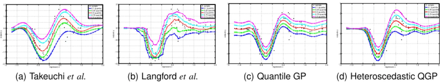
(a) Takeuchiet al. (b) Langfordet al. (c) Quantile GP (d) Heteroscedastic QGP
Figure 2. Illustration of conditional quantile analysis for Silverman’s motorcycle dataset via Quantile SVM (Takeuchiet al.), Reduction (Langfordet al.), Quantile GP, and Heteroscedastic QGP. The dataset exhibits heteroscedasticity. Non-crossing constraint is not enforced in Reduction and enforceable in Quantile SVM via additional linear constraints and is an inherent property of Quantile GP.
this sparse approximation in the California Housing dataset.
Input-dependent noise:We optimized the hyperparame-ters of both the noise-free and the noise process jointly using a scaled conjugate gradient approach. As locationsX¯ of the latent noise process, we selected 10 points linearly spaced in the bounding interval of the given input location.
Results: We run the linear model, SVM, learning reduc-tion, and Gaussian process methods for3 different quantile values for each dataset, i.e. at0.1,0.5and0.9. For Quantile SVM, we perform nested 5-fold cross-validation. There is no need to perform nested cross-validation for our approach, learning reduction approach, and the linear model as the free parameters are selected via log evidence, EP approximation of log evidence or there is no free parameter, respectively. The 5-fold cross validation results are summarized in Ta-ble II. Arguably, our estimator performs on par with (if not exceeding) state-of-the-art SVM and learning reduction based method. Noticeably, our approach has a competitive advantage over Quantile SVM for large datasets where the later approach might fail due to high memory and computational time requirements.
An illustration of the estimated quantile regression func-tions via SVM, learning reduction, and Gaussian process methods on the Motorcycle dataset is given in Figure 2.
VIII. CONCLUSIONS ANDFUTURERESEARCH We tackled the quantile estimation problem by modeling the conditional distribution and subsequently slicing the distribution at the respective quantile level to get the estimate of the latent quantile function. This approach is preferable when multiple quantile regression functions are needed and captures rather well the characteristics of the datasets.
In this paper, we have focussed on the specific example of Bayes quantile estimator, i.e. with Gaussian likelihood function. While this offers several appealing properties, the framework is by no means restricted to this. Our proposed Bayes quantile estimator offers two design parameters: like-lihood function (for robustness, a heavier tail distribution function might be more preferable) and non-parametric CDF (estimation of CDF directly from the data via residuals / errors).
ACKNOWLEDGMENT
The authors would like to thank Alex Smola, Marcus Hut-ter, and Marconi Barbosa for useful comments and sugges-tions. NICTA is funded through the Australian Government’s Backing Australia’s Ability initiative, in part through the ARC. The research was supported by the Pascal Network and the Fraunhofer ATTRACT fellowship STREAM.
REFERENCES
[1] C. Perlich, S. Rosset, R. D. Lawrence, and B. Zadrozny, “High-quantile modeling for customer wallet estimation and other applications,” inKDD ’07. ACM, 2007, pp. 977–985. [2] R. Koenker and G. Bassett, “Regression quantiles,”
Econo-metrica, vol. 46, no. 1, pp. 33–50, 1978.
[3] V. Vapnik, Estimation of Dependences Based on Empirical Data. Springer, 1982.
[4] C. Rasmussen, “Evaluation of Gaussian processes and other methods for non-linear regression,” Ph.D. dissertation, De-partment of Computer Science, University of Toronto, 1996,
http://www.kyb.mpg.de/publications/pss/ps2304.ps. [5] H. Nickisch and C. E. Rasmussen, “Approximations for
bi-nary gaussian process clasification,”JMLR, vol. 9, pp. 2035– 2078, 2008.
[6] J. Langford, R. Oliveira, and B. Zadrozny, “Predicting condi-tional quantiles via reduction to classification,” inUAI, 2006. [7] C. E. Rasmussen and C. K. I. Williams,Gaussian Processes for Machine Learning. Cambridge, MA: MIT Press, 2006. [8] R. Koenker, Quantile Regression. Cambridge University
Press, 2005.
[9] X. He, “Quantile curves without crossing,” The American Statistician, vol. 51, no. 2, pp. 186–192, may 1997. [10] I. Takeuchi, Q. V. Le, T. Sears, and A. J. Smola,
“Non-parametric quantile estimation,”J. Mach. Learn. Res., vol. 7, 2006.
[11] K. Yu and R. A. Moyeed, “Bayesian quantile regression,”
Statistics & Probability Letters, vol. 54, pp. 437–447, 2001. [12] J. Shim, C. Hwang, and K. H. Seok, “Non-crossing quantile regression via doubly penalized kernel machine,” in Compu-tational Statistics, vol. 24, 2009, pp. 83–94.