Modelling Systemic Risk using Neural Network Quantile Regression

(1)

Modelling Systemic Risk using Neural

Network Quantile Regression

Master Thesis submitted

to

Prof. Dr. Weining Wang

and

Prof. Dr. Wolfgang Karl Härdle

Humboldt-Universität zu Berlin

School of Business and Economics

Ladislaus-von-Bortkiewicz Chair of Statistics

by

Georg Keilbar

(546268)

in partial fulllment of the requirements

for the degree of

Master of Science in Economics

Berlin, July 9, 2018.

(2)

Abstract

We propose a novel approach to estimate the conditional value at risk (CoVaR) of nancial institutions. Our approach is based on neural network quantile regression. Building on the estimation results we model systemic risk spillover eects across banks by considering the marginal eects of the quantile regression procedure. We obtain a time-varying risk network represented by an adjacency matrix. We then propose three measures for systemic risk. The Systemic Fragility Index and the Systemic Hazard Index are measures to identify the most vulnerable and most critical rms in the nancial system, respectively. As a third risk measure we propose the Systemic Network Risk Index which represents the overall level of systemic risk. We apply our methodology to the global systemically relevant banks from the United States in a time period from 2007 until 2018. Our results are similar to previous studies about systemic risk. We nd that systemic risk increased sharply during the height of the nancial crisis in 2008 and again after a short period of easing in 2011 and 2015.

(3)

List of Abbreviations

ATAE Average tilted absolute error

CoVaR Conditional value at risk

G-SIB Global systemically important bank

iid independent and identically distributed

NNQR Neural network quantile regression

NYSE New York Stock Exchange

ReLU Rectier linear unit

RQEX Ratio of quantile exceedances

SFI Systemic Fragility Index

SHI Systemic Hazard Index

SNRI Systemic Network Risk Index

(5)

List of Figures

1 Neural network with a single hidden layer. . . 3

2 Architecture of a single neuron in a neural network . . . 4

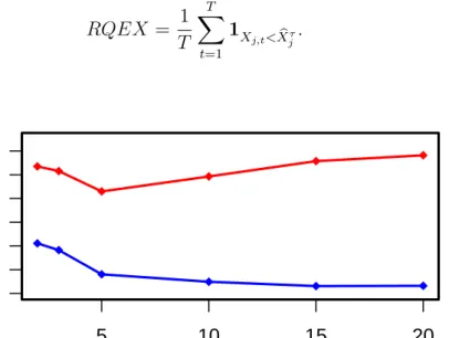
3 AT AE contingent on the number of hidden nodes. . . 16

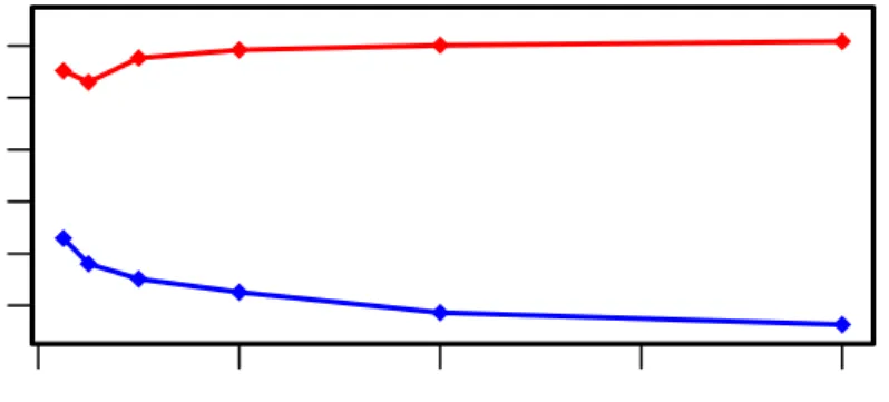
4 AT AE contingent on the number of epochs. . . 17

5 AT AE contingent on the dropout rate. . . 17

6 AT AE contingent on the elastic net parameters. . . 17

7 Returns, VaR and CoVaR . . . 19

8 Fitted neural network . . . 20

9 Level plot of average risk spillover eects . . . 21

10 Level plot of average risk spillover eects restricted to Lehman period . . . 21

11 Systemic risk network . . . 22

12 Systemic risk network after thresholding . . . 22

(6)

List of Tables

1 List of G-SIBs in the USA. . . 15 2 Performance measures for dierent model specications. . . 18 3 Firms ranked according to the systemic fragility index (averaged over

post-Lehman period). . . 23 4 Firms ranked according to the systemic hazard index. (averaged over

(7)

1 Introduction

The issue of systemic risk attracted a lot of attention from academics as well as from regulators in the aftermath of the nancial crisis of 2007-2009. Systemic risk refers to banks and other economic agents with substantial importance to the nancial system due to their size (too big to fail) or their centrality (too interconnected to fail). Conventional quantitative risk measures such as value at risk (VaR) are not suitable for capturing systemic risk adequately.

To tackle these issues, Adrian et al. (2016) [1] came up with conditional value at risk (CoVaR), a systemic extension of VaR. Their original approach is however restricted to analyze systemic risk in a bivariate context. Thus, Hautsch et al. (2014) [14] and Härdle et al. (2016) [10] extended the CoVaR framework further to analyze systemic risk in a multivariate and nonlinear context.

This master thesis oers a novel approach for the estimation of CoVaR using neural network quantile regression. Neural networks have become one of the most popular tools for prediction in recent years. They have been employed extensively and successfully to image classication as well as speech recognition problems. Our neural network based approach is highly suited for estimating CoVaR due to its exibility and nonparametric nature. Also it allows for a multivariate context.

In a rst step we estimated the VaR for each global systemically important nancial institution (G-SIB) from the United States by regressing their stock returns on a set of risk factors using linear quantile regression. Next we estimated the CoVaRs of the same rms using neural network quantile regression. Here we regressed the stock returns of each bank on the stock returns of the remaining banks. By approximating the conditional quantile with a neural network we ensure to capture possible nonlinear eects. In order to estimate risk spillover eects across banks we calculated the marginal eects by taking the derivative of the tted quantile with respect to the other banks' stock returns, evaluated at their VaR. By doing so we came up with a network of spillover eects represented by an adjacency matrix. This adjacency matrix is time-varying, i.e. we estimated a network for each trading day.

In a nal step we proposed three systemic risk measures building on the previous results. As a rst measure we proposed the Systemic Fragility Index which identies the most vulnerable banks in a given nancial risk network. The second measure is the Systemic Hazard Index which identies the nancial institutions which impose the biggest threat to the nancial system. These two measures characterize the rm-specic aspects of systemic risk. Thus we proposed a third measure which estimates the total level of systemic risk, the Systemic Network Risk Index.

(8)

Our estimation results show that systemic risk increased sharply during the height of the nancial crisis after the bankruptcy of Lehman Brothers in 2008. Systemic risk has stabilized over the last years with two minor spikes in 2011 and 2016. We have also identied the most systemically relevant nancial institutions during the nancial crisis.

The remainder of this thesis is organized as follows. Section 2 provides a brief introduction to neural networks in general and neural network quantile regression in particular. Section 3 describes in detail the methodology of this master thesis. After establishing the research framework step by step, we present the results in section 4. Section 5 discusses the results and concludes.

(9)

2 Neural Networks

2.1 Architecture of Neural Networks

A neural network is a nonlinear input-output model inspired by the processing of biological neurons in the human nervous system (Kuan et al., 1994 [22]). Mathematically, neural networks can be represented by a function, f : _Rp →_Rq_{, mapping from the input to the}

output space:

(y1, . . . , yq)> =f(x1, . . . , xp). (2.1)

Neural networks have a multiple-layer structure of directed graphs with one input layer, one or several hidden layer(s) and one output layer. While the input and output layers contain the input and output variables, respectively, the hidden layers function as inter-mediaries between those two. Neural networks are called feedforward since the directed graphs are acyclical.

Figure 1: Neural network with a single hidden layer.

An individual neuron is displayed by one node within a neural network. It can be repre-sented by a function, g :_RI _→

R, mapping from the input space to the one-dimensional

output space. Such a function has three tasks: weighting, aggregation and transformation of inputs. The optimal choice of weights will be explained in the next subsection. The aggregation is usually done by summation of weighted inputs. To introduce nonlinear eects, the aggregate is then transformed by an activation function, which often has a sigmoid shape (e.g. tanh(z)). In the recent past the rectier linear unit (ReLU) function,

max(0, z), became the most popular choice (Glorot et al., 2011) [9].

(10)

Figure 2: Architecture of a single neuron in a neural network [5].

exibility since no parametric structure has to be assumed on the functional relationship. The universal approximation theorem states that a feedforward neural network with at least one hidden layer and a nite number of hidden nodes is able to approximate any continuous function under some mild conditions on the activation function. Cybenko (1989) [6] provides a proof for the case of sigmoid activation functions.

Universal Approximation Theorem. Let σ be any continuous sigmoidal function.

Then nite sums of the form

G(x) =

n

X

j=1

αjσ(γj>x+θj)

are dense in C(In). In other words, given any f ∈C(In) and >0, there is a sum G(x)

in the above form, for which

|G(x)−f(x)|< for all x∈In.

While the universal approximation theorem makes a strong statement about the possi-bility of function approximation, it is silent on how to nd such an approximation. In particular it is silent about the required number of hidden nodes. And in general, the universal approximation theorem does not guarantee good results in practical applica-tions with limited data. Therefore the next subsection will explain methods for obtaining weights for a neural network.

Neural networks can be understood as a generalization of a standard regression problem (in the case of a continuous output variable) or a standard classication problem (in the case of a discrete output variable). But instead of using a linear equation the dependence of the output on the inputs is explained by a neural network. Nonlinearity is hereby introduced by the nonlinear transformation within the individual neurons and by the multiple-layer structure of the network. Linear regression is equivalent to neural network regression if the activation function is the identity for all nodes.

(11)

2.2 Learning in Neural Networks

The learning process of feedforward neural networks belongs to the paradigm of supervised learning (Hastie et al., 2009 [12]), so the teaching inputs include observed values of the independent variables as well as of the dependent variable.

For the training of neural networks linear optimization methods are no longer feasible. The most widely used estimation method for neural networks is the backpropagation algorithm (Werbos, 1974 [24] and Hinton et al., 1986 [15]). Backpropagation is an optimization method based on gradient descent.

Consider a neural network with one hidden layer, one output node, an activation function

g(·) and a quadratic loss functionL,

L(y,y_b) = n X 1=1 1 2(y−by) 2_, _(2.2)

whereyis the observed and_byis the tted value. The initial weights of the neural network

are chosen randomly but should be close to zero. The output is then obtained by passing the inputs forward through the network using the initial weights. Now the error can be calculated at the output node and also the gradient of the loss function with respect to the weights.

For the output layer the weight from a hidden node h is adjusted proportionally to its

derivative: ∆w_ho =−η ∂L ∂wo h (2.3) =−η(y−y_b)g0 M X m=1 wh_mom ! oh, (2.4)

with oh being the output of the hidden layer neuron h, M is the number of hidden nodes

and η is the learning rate.

Hidden layer weights are also adjusted according to the gradient. Since the error is brought backward through the network the weight adjustment depends on the adjustments at subsequent nodes. The weight between an input j and hidden node h is adjusted in the

following way: ∆wh_j,h =−η ∂L ∂wh j,h (2.5) =−ηw_hoδog0 K X i=1 wh_i,hxi ! xj, (2.6)

(12)

where δo = (y−by)g 0 M X m=1 wh_mom ! (2.7) and xj represents the j-th input and K is the number of input variables.

This procedure of propagation of the error and subsequent weight adjustment is repeated until a stopping criterion is fullled. This can be a predened number of maximal itera-tions or a threshold for the loss function.

Algorithm 1 Backpropagation

1: Initialize network weights randomly 2: repeat

3: for all Training examples do

4: Propagation of the input to obtain the output of the neural network

5: Calculate the error

6: Pass the error back through the network

7: Update the weights according to the gradient of the error

8: until No. iterations > max no. of iterations OR other stopping criterion

In standard gradient descent the whole sample is used to calculate the gradient based on the forward propagation of inputs. However, when the sample size becomes large, this is no longer ecient. Therefore it might be preferable to consider mini batches (randomly selected cases) for each iteration of forward- and backpropagation (Hardt et al., 2016 [11]). This method is called stochastic gradient descent.

The practical problem of gradient-based methods is that it might be dicult to nd a global minimum. This problem can be induced by the existence of local minima and saddle points. The algorithm might stop early if the gradient of the error is close to zero, i.e. a marginal change in the weights does not have a signicant impact on the error. Several optimization algorithms have come up with solutions to these practical problems. A possible remedy is to consider an adaptive learning rate η for every parameter and at

each time step. Another method is to introduce momentum for the learning rate in order to avoid being stuck in local minima. Current gradient-based optimization algorithms are ADADELTA (Zeiler, 2012 [25]) and ADAM (Ba, 2015 [2]).

2.3 The Bias-Variance Trade-o

A central issue of neural networks and machine learning in general is overtting. One has to be very careful with the choice of tuning parameters, such as the number of hidden layers or the number of hidden nodes. If the architecture of the neural network is too

(13)

complex, there is a tendency to not only t the structure of the data but also the noise. As a consequence, the training error can be reduced to zero but the model typically generalizes poorly.

Predictive accuracy can be measured by the expected prediction error (Hastie et al., 2009 [12]):

Err = E [L{Y, f(X)}], (2.8)

where L(·) is an arbitrary loss function. However, neural networks minimize only the

training error which is an overly optimistic approximation of the actual expected pre-diction error. This optimism lies in the repeated use of the data for estimation and evaluation. err = 1 N N X i=1 LnYi,fb(X_i) o (2.9) Under the assumption of a quadratic loss function and by xing the covariates (X =x0),

the expected prediction error can be decomposed in the following way:

Err(x0) =σ2+ Bias 2n b f(x0) o + Varnbf(x₀) o . (2.10)

Predictive accuracy is thus determined by the bias as well as the variance of the model. The rst term, σ2

, is the irreducible error which is independent of any model.

Neural networks with a suciently complex structure are able to reduce the bias to zero at the expense of a high variance. A simple way to mitigate this problem is to introduce an additional penalty term for model complexity. Common choices are weight decay (L2)

and LASSO (L1_{) penalization on the weights.}

Hastie et al. (2005) [13] propose elastic net, a L1_/_L2 _{hybrid penalization. When}

consid-ering an arbitrary loss function L(·), the optimization problem becomes:

min

θ L(θ) +λ

(1−α)kθk1 +αkθk22 , (2.11)

where θ is a vector of parameters. If α= 0, elastic net is identical to LASSO, if α= 1, it

is identical to weight decay penalization. The advantage of elastic net is that it achieves the sparsity property of the LASSO and works well with highly correlated regressors. However, feature selection is not really possible in the context of neural networks, due to their multiple-layer structure. A particular input variable has multiple weights and a shrinkage of one weight to zero does not eliminate the whole variable but only one connection of the neural network.

(14)

The currently most prevalent regularization method for neural networks is dropout (Hin-ton et al., 2014 [16]). The idea is to randomly drop units with a probability pand adjust

the weights for a thinned-out network. The nal trained model can then be seen as an ensemble of less complex neural networks. Dropout tries to mitigate the risk of co-adaptation of weight parameters, which can be the cause for overtting (Hinton et al., 2012 [17]).

2.4 Neural Network Quantile Regression

Neural networks have been applied extensively to mean regression and classication prob-lems. Neural networks can also be used for approximating quantiles. This was rst formalized by Taylor (2000) [23]. An application to time series data can be found in Xu et al. (2016) [18], who extended the CaViaR framework of Engle et al. (2004) [8] by using neural network quantile regression instead of standard quantile regression.

Conceptually, the approach is similar to linear quantile regression, as introduced by Koenker et al. (1978 [19], 1982 [20]). The goal is to nd the best approximation for the conditional quantile of a random variable. Therefore the following loss function has to be minimized: min θ T X t=1 ρτ{yt−yb τ t(θ)}, (2.12)

where θ is a vector of coecients, yt are the observed values and yb

τ

t(θ) are the tted τ-quantiles and ρτ is the tilted absolute error function dened as:

ρτ(u) =    τ u if u≥0 (τ −1)u if u <0 , (2.13)

Since the backpropagation algorithm requires dierentiability, Taylor (2000) proposes a slight modication of the loss function:

ρτ(u) =    τ h(u) if u≥0 (τ −1)h(u) if u <0 , (2.14)

with h(u) being the Huber norm, a hybrid L1/_L₂norm, dened as: h(u) =    u2 2 if 0≤ kuk ≤ kuk − 2 if kuk> . (2.15)

(15)

The functional form of a neural network quantile regression model with one hidden layer is given by f(Xt,w) = M X m=1 wo_m g K X k=1 w_k,mh Xk,t+bhm ! +bo, (2.16)

wherewh_k,mis the weight from inputk to hidden nodem,wh_m is the weight of hidden node m and bh_m and bo are the corresponding bias terms for the hidden nodes and the output

node. g(·)is a nonlinear hidden layer activation function. The activation function for the

output node is assumed to be linear.

The estimated conditional τ-quantile is then the tted value of the neural network:

b

Y_tτ =f(xt,wb), (2.17)

wherew is the solution of the backpropagation procedure andb xtis the vector of all inputs at time t.

Neural network quantile regression as dened above was implemented in R in the QRNN package (Cannon, 2011) [3]. The package also allows for the inclusion of a L2 penalty

term. Recent software packages do not require dierentiability of the loss function and also enables the consideration of more complex neural networks.

(16)

3 Methodology

In this section we explain the details of our systemic risk analysis. Our methodology involves four steps. The rst step is concerned with the estimation of VaR with linear quantile regression using a set of risk factors as explaining variables. The results are used in the next step to estimate the CoVaR for each nancial institution using neural network quantile regression. Next we calculate marginal eects to model systemic risk spillover eects, resulting in a time-varying systemic risk network. In the nal step we propose three systemic risk measures based on this systemic risk network.

3.1 Step 1: Estimation of VaR

VaR is dened as the maximum loss over a xed time horizon at a certain level of con-dence. Mathematically, it is the τ-quantile of the prot and loss distribution:

P(Xi,t ≤VaRτi,t) =τ, (3.1)

where Xi,t is the return of rmi at timet and τ ∈(0,1)is the quantile level.

The VaR of each rm i is estimated as the tted value of a linear quantile regression

procedure by regressing the returns on a set of macro state variables Mt−1.

Xi,t =αi+γiMt−1+i,t, (3.2)

where the conditional quantile of the error termτ

i,t|Mt−1 = 0. The VaR is the tted value

of the linear quantile regression problem:

VaRτ_i,t =α_bi+bγiMt−1. (3.3)

3.2 Step 2: Estimation of CoVaR with NNQR

CoVaR was introduced as a systemic extension for standard VaR (Adrian et al., 2016 [1]). Similar to VaR, it is a risk measure dened as a conditional quantile of the loss distribution. But deviating, CoVaR is contingent on a specic nancial distress scenario. The motivation for using CoVaR is the identication of systemically important banks. For the distress scenario we assume that all other rms are at their VaR. By doing this we follow the reasoning of Hautsch et al. (2014) [14] and Härdle et al. (2016) [10].

(17)

where X−j,t is a vector of returns of all rms except j and VaRτ−j,t is the corresponding

vector of VaRs.

CoVaR can be estimated as a tted conditional quantile, building on the results for the VaRs obtained in step 1. Chao et al. (2015) [4] and Härdle et al. (2016) [10] nd evidence for nonlinearity in the dependence between pairs of nancial institutions. Hence, linear quantile regression might not be an appropriate procedure to estimate the risk spillovers. We therefore propose the use of neural network quantile regression. The exibility of the approach allows to detect possible nonlinear dependencies in the data.

The conditional quantile of bank j's returns is regressed on the returns of all other banks

and using a neural network as dened in section 2.4:

Xj,t =f(X−j,t,w) +j,t, (3.5) = M X m=1 w_mo g K X k6=j wh_k,mXk,t+bhm ! +bo+j,t, (3.6)

with the conditional quantile of error term τ_j,t|X−j,t = 0.

To calculate the CoVaR of rm j, the tted neural network has to be evaluated at the

distress scenario:

CoVaRτ_j,t =f(VaRτ₋_j,t,w_b), (3.7)

where w is the estimated vector of weights and bias terms. Nonlinearity is introduced byb the use of the nonlinear activation function.

3.3 Step 3: Calculation of Risk Spillover Eects

Based on the weights estimated by the NNQR procedure, it is now possible to obtain risk spillover eects between each directed pair of banks. We propose to estimate the spillover eects by taking the rst derivative of the conditional quantile of rm j's return with

respect to the return of rm i. ∂Xτ j|−j,t ∂Xi,t = ∂ ∂Xi,t M X m=1 wo_m g K X k6=j w_k,mh Xk,t+bhm ! +bo+j,t (3.8)

In the case of a sigmoid tangent activation function we have

∂Xτ j|−j,t ∂Xi,t = M X m=1 w_mow_i,mh g0 K X k6=j wh_k,mXk,t+bhm ! (3.9)

(18)

with

g0(z) = ∂tanh(z/2)

∂z (3.10)

= 2

(exp−z/2_{+ exp}z/2₎2. (3.11)

In the case of a ReLu activation function we have

∂X_jτ_|−_j,t ∂Xi,t = M X m=1 wo_mw_i,mh 1 K X k6=j wh_k,mXk,t+bhm >0 ! . (3.12)

Since we are interested in the lower tail dependency, we consider the marginal eect evaluated at the distress scenario as dened in the previous subsection:

∂CoVaRτ j,t ∂VaRτ_i,t = M X m=1 wo_mw_i,mh g0 K X k6=j wh_k,mVaRk,t+bhm ! . (3.13)

Calculating such a marginal eect for each directed pair of rms yields an o-diagonal adjacency matrix of risk spillover eects at time t:

At=       0 a12,t . . . a1K,t a21,t 0 . . . a2K,t ... . . . ... ... aK1,t aK2,t . . . 0       , (3.14)

with elements dened as absolute values of marginal eects:

aji,t =    |∂CoVaR τ j,t ∂VaRτ i,t |, if j 6=i 0, if j =i . (3.15)

Note that the risk spillover eects are not symmetric in general, thus aji,t 6= aij,t. This

adjacency matrix species a weighted directed graph modeling the systemic risk in the nancial system.

3.4 Step 4: Network Analysis of Spillover Eects

To further analyze the systemic relevance of the nancial institutions we can calculate several network measures proposed by Diebold et al. (2014) [7].

(19)

absolute marginal eects of all other rms on j. Cj←·,t = K X i=1 aji,t (3.16)

Analogously, one can dene the total directional connectedness from rm i at time t as

the sum of absolute marginal eects from i to all other rms. C·←i,t =

K

X

j=1

aji,t (3.17)

Lastly, Diebold et al. dene the total connectedness at time t as the sum of all absolute

marginal eects. Ct= 1 K K X i=1 K X j=1 aji,t (3.18)

The total connectedness is a measure for the interconnectedness on the level of the entire system, without dierentiating between individual components of the network.

Building on the analysis of Diebold et al., we rene the approach by incorporating VaR and CoVaR in the measurement of the systemic relevance. In particular, we propose the Systemic Fragility Index (SFI) and the Systemic Hazard Index (SHI):

SF Ij,t = K X i=1 1 +|VaRτ_i,t| ·aji,t (3.19) SHIi,t = K X j=1 1 +|CoVaRτ_j,t| ·aji,t (3.20)

The SFI is a systemic risk measure for the vulnerability of a nancial institution. It increases if those adjacency weights pointing to j are large and also if the VaRs of rms i (i.e. the risk factors for j) increase.

The SHI is a risk measure for the exposure of the nancial system to rm i. It depends

on the out-going adjacency weights from i and also on the other rm's CoVaR.

As a third index we propose the Systemic Network Risk Index (SNRI), a measure for the total systemic risk in the nancial system which depends on the marginal eects, the outgoing VaRs and the incoming CoVaRs.

(20)

SN RIt= K X i=1 K X j=1

(1 +|VaRτ_i,t|)·(1 +|CoVaRτ_j,t|)·aji,t. (3.21)

Lastly, we dene the adjusted adjacency matrix,

e At=       0 _ea12,t . . . ea1K,t ea21,t 0 . . . ea2K,t ... . . . ... ... e aK1,t eaK2,t . . . 0       , (3.22)

with elements dened as:

eaji,t =  



aji,t·VaRτi,t·CoVaR τ

j,t, if j 6=i

0, if j =i

. (3.23)

The adjusted adjacency matrix accounts for the level of outgoing VaRs and incoming CoVaRs and is an improved representation of risk spillover eects. Systemic spillover eects are thus determined by the marginal eects of the NNQR procedure as well as by the VaRs and CoVaRs.

(21)

4 Results

4.1 Data

The data contains stock returns for the global systemically important banks (G-SIBs) from the United States selected by the Financial Stability Board (FSB) in the time period between January 4, 2007 and May 31, 2018. The daily stock returns are obtained from Yahoo Finance.

Financial Institution NYSE symbol

Wells Fargo & Company WFC

JP Morgan Chase & co. JPM

Bank of America Corporation BAC

Citygroup C

The Bank of New York Mellon Corporation BK

State Street Corporation STT

Goldman Sachs Group, Inc. GS

Morgan Stanley MS

Table 1: List of G-SIBs in the USA.

Additionally to these return data, we consider daily observations of the following set of macro state variables.

i) implied volatility index (VIX), from Yahoo Finance; ii) the weekly S&P500 index returns, from Yahoo Finance;

iii) Moody's Seasoned Baa Corporate Bond Yield Relative to Yield on 10-Year Treasury Constant Maturity from Federal Reserve Bank of St. Louis;

iv) 10-Year Treasury Constant Maturity Minus 3-Month Treasury Constant Maturity from Federal Reserve Bank of St. Louis.

4.2 Model Selection

The tuning parameters for the neural network quantile regression procedure are selected in the following way. For each nancial institution we regress the returns on the other rms' returns to estimate the 5% quantile. The data is separated into a training and a validation set repeatedly in a moving window approach. We consider an estimation window of 250 days and a subsequent validation window of 50 days. Start of each estimation window is the begin of the new year. The resulting performance indicators are then aggregated over all rms and all windows to select the best model.

(22)

As a rst measure for model performance we propose the average tilted absolute error of prediction (AT AE) which can be compared to the MSE in mean regression:

AT AE = 1 T T X t=1 ρτ(Xj,t−Xb_j_|−_j,t), (4.1)

where Xj,t is the observed and Xb_jτ_|−_j,t the tted value. A small value for the AT AE is preferred.

The second measure is the R1 criterion (Koenker et al., 1999 [21]), a coecient of

deter-mination dened analogously to the R2 _{measure in mean regression.} R1 = 1− PT t=1ρτ(Xj,t−Xb τ j|−j,t) PT t=1ρτ(Xj,t−Xb_jτ) , (4.2)

where Xb_jτ is the estimated unconditional τ-quantile. It should be noted that for the in-sample t it has to hold that R1 _∈ _[0_,_1]. However, the out-of-sample t for a particular

unsuitable model can be worse than a constant unconditional quantile t. In this case the R1 can even be negative.

Lastly, we introduce the ratio of quantile exceedances (RQEX) as a measure of

calibra-tion. A well-calibrated model should have a ratio close to τ: RQEX = 1 T T X t=1 1_X j,t<Xb_jτ. (4.3) 5 10 15 20 0.0012 0.0020 A T AE

Figure 3: AT AE contingent on the number of hidden nodes. In-sample t (blue line) and

(23)

0 200 400 600 800 0.0012 0.0020 A T AE

Figure 4: AT AE contingent on the number of epochs. In-sample t (blue line) and

out-of-sample t (red line).

Figures 3 and 4 visualize the problems of overtting. A large number of hidden nodes and a large number of epochs can eectively reduce the training error (blue line). However, the test error (red line) decreases only to a certain point. After this point the test error starts to increase again.

0.0 0.1 0.2 0.3 0.4 0.5 0.0014 0.0020 A T AE

Figure 5: AT AE contingent on the dropout rate p. In-sample t (blue line) and

out-of-sample t (red line).

0.0 0.2 0.4 0.6 0.8 1.0 0.00200 0.00210 A T AE

Figure 6: AT AE contingent on elastic net parameterα. λ= 0.0001(solid line),λ= 0.001

(24)

We considered two dierent regularization methods, dropout and elastic net. The results are shown in Figures 5 and 6. A small dropout rate (10-20%) can reduce the test error compared to the baseline setting of zero dropout. Elastic net penalization can also improve the t, given thatλis not chosen to be too large. Both methods have, however, a negative

impact on the in-sample t, as they introduce a bias to the model.

For model selection we consider 10 dierent model specications. The results can be found in Table 2 1_. Model AT AE R1 RQEX ReLu, H = 5 0.002026 0.4668 0.0650 ReLu, H = 5,α = 0, λ= 0.001 0.002026 0.4675 0.0661 ReLu, H = 5,α = 0.25,λ = 0.001 0.002023 0.4682 0.0657 ReLu, H = 5,p= 0.1 0.001973 0.4728 0.0595 ReLu, H = 5,α = 0.25,λ = 0.001, p= 0.1 0.001973 0.4740 0.0584 ReLu, H = (5,2), p= 0.1 0.002193 0.4554 0.0770 ReLu, H = (3,3), p= 0.1 0.002227 0.4412 0.0677 ReLu, H = 10,p= 0.1 0.002033 0.4788 0.0752 tanh, H = 2 0.002845 0.3030 0.1018 tanh, H = 5 0.002643 0.3691 0.1036

Table 2: Out-of-sample performance for dierent model specications. We consider ReLu and tanh activation functions, H refers to the number and structure of hidden nodes, α

and λ are the elastic net parameters andp is the input layer dropout rate.

The results in Table 2 suggest that complex models are dominated by less complex models. As a second observation, the ReLu (rectier linear unit) activation function is superior to the tanh activation function. Both dropout and elastic net have a positive impact on the model performance.

The best model of the candidates is a neural network with 5 hidden nodes in a single hidden layer with a ReLu activation function. The model has also a dropout ratio of

p= 0.1 and elastic net parameters α= 0.25and λ= 0.001. It ranks rst inAT AE (one

of only two models that fall below 0.002) and second in R1_{. Also the model's} _RQEX

(0.0584) is the closest to the quantile level of 0.05. We will use this model in the following estimation steps.

1_{We use the ADADELTA optimization algorithm with parameters} _ρ _{= 0}_.₉₉ _and _{= 1}_e₋₀₈_{. The}

(25)

4.3 Estimation Results

4.3.1 VaR and CoVaR

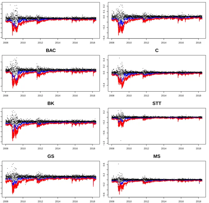
As explained in section 3, the analysis is carried out in four steps. In the rst two steps VaR and CoVaR are estimated for each rm, using linear quantile regression and neural network quantile regression, respectively. To account for potential non-stationarity, we employ a sliding window estimation framework for both measures. The window size is chosen to be 250 observations (implying one year of daily stock returns). We chose the quantile level τ = 5%. The tted values for all banks are visualized in Figure 7.

2008 2010 2012 2014 2016 2018 −0.4 −0.2 0.0 0.2 WFC date[−c(1:250)] 2008 2010 2012 2014 2016 2018 −0.4 −0.2 0.0 0.1 0.2 JPM date[−c(1:250)] 2008 2010 2012 2014 2016 2018 −0.4 −0.2 0.0 0.2 BAC date[−c(1:250)] 2008 2010 2012 2014 2016 2018 −0.4 0.0 0.2 0.4 C date[−c(1:250)] 2008 2010 2012 2014 2016 2018 −0.4 −0.2 0.0 0.2 BK date[−c(1:250)] 2008 2010 2012 2014 2016 2018 −1.0 −0.6 −0.2 0.2 STT date[−c(1:250)] 2008 2010 2012 2014 2016 2018 −0.3 −0.1 0.1 0.2 GS 2008 2010 2012 2014 2016 2018 −0.6 −0.2 0.2 0.6 MS

Figure 7: Plot of Returns (black dots), VaR (blue line) and CoVaR estimated by NNQR (red line).

(26)

The VaRs and CoVaRs of all banks follow a similar pattern. In the course of the nancial crisis and the bankruptcy of Lehman Brothers and Bear Stearns, both measures explode, indicating an increase in systemic risk during this period. After a short stabilization period, the CoVaRs rise again in the second half of 2011. What follows is a relatively stable period with a few non-persistent spikes.

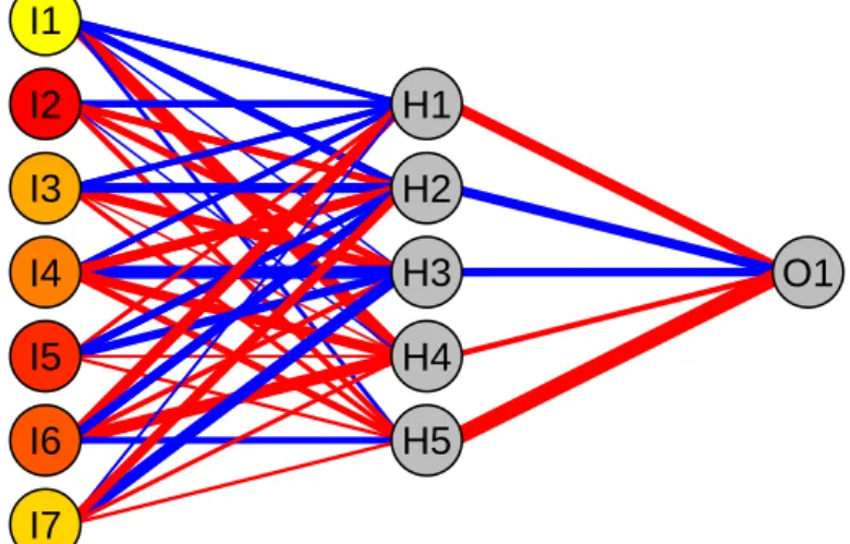
I1 I2 I3 I4 I5 I6 I7 WFC JPM BAC C BK STT GS H1 H2 H3 H4 H5 O1 MS

Figure 8: Fitted quantile regression neural network for Morgan Stanley on March 13, 2008. Red connections indicate negative weights, blue connections indicate positive weights. The color of the input nodes visualizes the variable importance rank calculated as the marginal eect of the respective rm on Morgan Stanley (yellow implies low importance, red implies high importance).

4.3.2 Risk Spillover Network

Based on the weights estimated in the NNQR procedure and the estimated VaRs and CoVaRs, we calculated the spillover of each pair of banks for each point in time of the estimation horizon. The result is a time-varying weighted adjusted adjacency matrix (as dened in equation 3.22). Figure 9 visualizes a simple time average of these matrices.

(27)

WFC JPM BAC C BK STT GS MS WFC JPM BAC C BK STT GS MS 0.0 0.1 0.2 0.3 0.4 0.5 0.6 0.7

Figure 9: Level plot of the risk spillover eects, averaged over the whole estimation period.

WFC JPM BAC C BK STT GS MS WFC JPM BAC C BK STT GS MS 0.0 0.1 0.2 0.3 0.4 0.5 0.6 0.7

Figure 10: Level plot of the risk spillover eects, averaged over post-Lehman period (September 15, 2008 - December 14, 2008).

When restricting the included observations to the period up to three months after the Lehman bankruptcy, the time average looks dierently. Figure 10 shows that the spillover eects were signicantly larger during this period of nancial distress. This result is in line with economic theory, as nancial institutions were in fact very interconnected due to large derivative positions causing mutual counterparty risk.

Another important observation that can be made from these two plots is that the spillover eects have a tendency to be symmetric. If one bank has a large impact on another bank, the converse is also likely. This symmetry pattern becomes even more clear when looking at the network representations of the spillover eects in Figures 11 and 12. The largest edges (30%) of the network, as visualized in Figure 12, occur mostly in pairs. The symmetry is not caused by the model setup, which is asymmetric in its nature, but is rather implied by the data.

(28)

WFC JPM BAC C BK STT GS MS

Figure 11: Systemic Risk network of spillover eects, averaged over the whole estimation period. WFC JPM BAC C BK STT GS MS

Figure 12: Systemic Risk network of spillover eects, averaged over the whole estimation period. Only the 30% largest edges are displayed.

(29)

4.3.3 Network Risk Measures

Finally, we estimated the systemic network measures using the results of the previous steps. The Systemic Network Risk Index is a measure for the overall systemic risk in the nancial system. The time series plot can be found in Figure 13. From 2008 until the start of 2018 there have been one large and two smaller spikes. The rst and largest spike represents the height of the nancial crises. Two smaller ones follow in 2011/2012 and 2015/2016, each. 2008 2010 2012 2014 2016 2018 15 20 25 30

Figure 13: Systemic Network Risk Index (grey line) and cubic spline interpolation with sparsity parameter equal to 0.8 (blue line).

Rank Bank SF I 1 STT 2.433 2 BK 2.362 3 BAC 2.225 4 MS 2.233 5 JPM 2.134 6 C 2.125 7 GS 2.069 8 WCF 2.019

Table 3: Firms ranked according to the systemic fragility index (averaged over post-Lehman period).

Rank Bank SHI

1 BAC 2.730 2 GS 2.431 3 MS 2.372 4 BK 2.342 5 C 2.289 6 JPM 2.221 7 WCF 2.211 8 STT 2.041

Table 4: Firms ranked according to the systemic hazard index. (averaged over post-Lehman period).

While the SN RI does not dierentiate between dierent banks, we then identied the

most systemically relevant rms during the nancial crises. Hereby we considered the most vulnerable banks identied by the SF I in Table 3 as well as the most dangerous

(30)

banks identied by theSHI in Table 4. The results in the tables represent averages over

the three month period after the Lehman bankruptcy.

The most fragile banks according to our methodology are the State Street Corporation, the The Bank of New York Mellon Corporation and the Bank of America Corporation. The rms which impose the largest systemic risk to the nancial system are again the Bank of America Corporation, Goldman Sachs and Morgan Stanley. While Goldman Sachs ranks very high in the SHI, it is nearly at the bottom of theSF I, indicating that their

exposure to the nancial system is weaker than the other way around. The opposite is the case for the State Street Corporation which has the largest SF I and the lowest SHI

(31)

5 Conclusion

Even if the global economy seems to have recovered from the nancial crisis, systemic risk is still a relevant topic. Whereas there are no immediate systemic threats to the nancial system today, latent risks are still present.

This master thesis proposes a novel approach to estimate the conditional Value at Risk (CoVaR) of nancial institutions based on neural network quantile regression. We esti-mate a network of systemic risk spillover eects and propose three network-based risk measures, the Systemic Fragility Index to rank the rms with the largest exposure to the nancial system, the Systemic Hazard Index which ranks the rms according to the risks they impose to the nancial system and the Systemic Network Risk Index which is a measure for the overall systemic risk.

The methodology is applied to the global systemically important banks from the United States in the period from 2007 until 2018. The results are in line with previous ndings in the literature. We observe the Systemic Network Risk Index increasing sharply during the nancial crisis after which it stabilizes.

This master thesis is an important contribution to the vast literature about systemic risk. Neural networks have been utilized almost exclusively as a device for prediction. An accomplishment of this thesis is to nd a way to interpret the underlying neural network by estimating risk spillover eects out of the tted neural networks.

We leave it open for future research to investigate possible benets of connecting the estimation of CoVaR in the cross-sectional and the time series dimension. Our current methodology treats the single estimation problems separately from each other. Recent advances in transfer learning and multitask learning suggest that this is promising research path to increase eciency.

(32)

References

[1] Adrian, T. and Brunnermeier, M.K., (2016). CoVaR. American Economic Review vol. 106, no. 7, (pp. 1705-41).

[2] Ba, J. and Kingma, P., (2015). ADAM: A Method for Stochastic Optimization. Pub-lished as a conference paper at ICLR 2015.

[3] Cannon, A.J. (2011). Quantile regression neural networks: Implementation in R and application to precipitation downscaling. Computers & Geosciences 37, 1277-1284. [4] Chao, S.-K., Härdle, W.K., Wang, W., 2015. Quantile regression in risk calibration.

Handb. Financ. Econom. Stat. 1467-1489.

[5] Chrislb, 2005. Figure retrieved from https://commons.wikimedia.org/wiki/ File:ArticialNeuronModel_english.png on June 15, 2018.

[6] Cybenko, G. (1989). Approximation by Superpositions of a Sigmoidal Function. Math. Control Signals Systems (1989) 2:303-314.

[7] Diebold, F.X. and Yilmaz, K. (2014). On the network topology of variance decompo-sitions: Measuring the connectedness of nancial rms. Journal of Econometrics 182, 119-134.

[8] Engle, R.F. and Manganelli, S. (2004). CAViaR, Journal of Business & Economic Statistics, 22:4, 367-381, DOI:10.1198/073500104000000370.

[9] Glorot, X., Bordes, A. and Bengio., Y. Deep sparse rectier neural networks (2011). In Proc. 14th International Conference on Articial Intelligence and Statistics, 315-323. [10] Härdle, W.K., Wang, W. and Yu, L. (2016). TENET: Tail-Event driven NETwork

risk. Journal of Econometrics, Volume 192, Issue 2, Pages 499-513.

[11] Hardt, M., Recht, B. and Singer, Y. Train faster, generalize better: Stability of stochastic gradient descent. arXiv, 1509.01240, 2015.

[12] Hastie, T., Tibshirani, A. and Friedman, J. (2009). The Elements of Statistical Learn-ing (2. Edition). Stanford, SprLearn-inger.

[13] Hastie, T. and Zou, H. (2005). Regularization and variable selection via the elastic net. J. R. Statist. Soc. B, 67, Part 2, pp. 301-320.

[14] Hautsch, N., Schaumburg, J. and Schienle, M. (2014). Financial Network Systemic Risk Contributions. Review of Finance, Volume 19, Issue 2, 1 March 2015, Pages 685-738.

(33)

[15] Hinton, G.E., Rumelhart, D.E. and Williams, R.J. (1986). Learning representations by back-propagating errors. Nature (1986) Band 323, S. 533-536.

[16] Hinton, G.E., Krizhevsky, A., Salakhutdinov, R., Srivastava, N. and Sutskever, I. (2014). Dropout: A Simple Way to Prevent Neural Networks from Overtting. Journal of Machine Learning Research, 15, 1929-1958.

[17] Hinton, G.E., Krizhevsky, A., Salakhutdinov, R., Srivastava, N. and Sutskever, I. (2012). Improving neural networks by preventing co-adaptation of feature detectors. arXiv: 1207.0580.

[18] Jiang, C., Liu, X., Xu, Q., and Yu, K. (2016). Quantile autoregression neural network model with applications to evaluating value at risk. Applied Soft Computing 49, 1-12. [19] Koenker, R.W. and Bassett, G.W. (1978). Regression Quantiles, Econometrica, 46,

33-50.

[20] Koenker, R.W. and Bassett, G.W. (1982). Robust Tests for Heteroscedasticity Based on Regression Quantiles. Econometrica 50, 43-62.

[21] Koenker, R.W. and Machado J.A.F. (1999). Goodness of t and related inference processes for quantile regression, J. Amer. Statist. Assoc. 94(448), pp. 1296-1310. [22] Kuan, C.-M. and White, H. (1994). Articial neural networks: an econometric

per-spective. Econometric Reviews, 13:1, 1-91, DOI: 10.1080/07474939408800273.

[23] Taylor, J.W. (2000). A Quantile Regression Neural Network Approach to Estimating the Conditional Density of Multiperiod Returns. Journal of Forecasting, Vol. 19, pp. 299-311.

[24] Werbos, P. (1974). Beyond regression: new tools for prediction and analysis in the behavioral sciences. PhD thesis, Harvard University, Cambridge, Nov. 1974.

[25] Zeiler, M. D. (2012). ADADELTA: An adaptive learning rate method. arXiv: 1212.5701., 2012.

(34)

Declaration of Authorship

I hereby conrm that I have authored this Master's thesis independently and without use of others than the indicated sources. All passages which are literally or in general matter taken out of publications or other sources are marked as such.

Berlin, July 9, 2018