SVM-Maj: A Majorization Approach to Linear
Support Vector Machines with Different Hinge
Errors
P.J.F. Groenen
∗G. Nalbantov
†J.C. Bioch
‡November 1, 2007
Econometric Institute Report EI 2007-49 Abstract
Support vector machines (SVM) are becoming increasingly popular for the prediction of a binary dependent variable. SVMs perform very well with respect to competing techniques. Often, the solution of an SVM is obtained by switching to the dual. In this paper, we stick to the primal support vector machine (SVM) problem, study its effective aspects, and propose varieties of convex loss functions such as the standard for SVM with the absolute hinge error as well as the quadratic hinge and the Huber hinge errors. We present an iterative majorization algorithm that minimizes each of the adaptations. In addition, we show that many of the features of an SVM are also obtained by an optimal scaling approach to regression. We illustrate this with an example from the literature and do a comparison of different methods on several empirical data sets.
Keywords: Support vector machines, Iterative majorization, I-Splines, Absolute hinge error, Quadratic hinge error, Huber hinge error, Optimal scaling.
1
Introduction
In recent years, support vector machines (SVMs) have become a popular tech-nique to predict two groups from a set of predictor variables (Vapnik, 2000). This data analysis problem is not new and such data can also be analyzed
∗Econometric Institute, Erasmus University Rotterdam, P.O. Box 1738, 3000 DR
Rotter-dam, The [email protected]
†ERIM and Econometric Institute, Erasmus University Rotterdam, P.O. Box 1738, 3000
DR Rotterdam, The [email protected]
‡Econometric Institute, Erasmus University Rotterdam, P.O. Box 1738, 3000 DR
through alternative techniques such as linear and quadratic discriminant anal-ysis, neural networks, and logistic regression. However, SVMs seem to compare favorably in their prediction quality with respect to competing models. Also, their optimization problem is well defined and can be solved through a quadratic program. Furthermore, the classification rule derived from an SVM is relatively simple and it can be readily applied to new, unseen samples. At the downside, the interpretation in terms of the predictor variables in nonlinear SVM is not always possible. In addition, the usual dual formulation of an SVM may not be so easy to grasp.
In this paper, we offer a different way of looking at linear SVMs that makes the interpretation easier. First of all, we stick to the primal problem and for-mulate the SVM in terms of a loss function that is regularized by a penalty term. From this formulation, it can be seen that SVMs use robustified errors. Apart from the standard SVM loss function that uses the absolute hinge error, we introduce two other hinge errors, the Huber and quadratic hinge errors, and show the relation with ridge regression.
The second theme of this paper is to show the connection between optimal scaling regression and SVMs. The idea of optimally transforming a variable so that a criterion is being optimized has been around for more than 30 years (see, for example, Young, 1981; Gifi, 1990). We show that optimal scaling regression using an ordinal transformation with the primary approach to ties comes close to the objective of SVMs. We discuss the similarities between both approaches and give a formulation of SVM in terms of optimal scaling.
A third theme is to propose a new majorization algorithm that minimizes the loss for any of the hinge errors. The advantage of majorization is that each iteration is guaranteed to reduce the SVM loss function until convergence is reached. Finally, we provide numerical experiments on a suite of 14 empirical data sets to study the predictive performance of the different errors in SVMs and compare it to optimal scaling regression. We also compare the computational efficiency of the majorization approach for the SVM to several standard SVM solvers.
Note that this paper is a significantly extended version of Groenen, Nalban-tov, and Bioch (2007).
2
The SVM Loss Function
In many ways, an SVM resembles regression quite closely. Let us first introduce some notation. LetXbe then×m matrix of predictor variables ofnobjects andmvariables. The n×1 vectorycontains the grouping of the objects into two classes, that is, yi = 1 if objecti belongs to class 1 andyi =−1 if object
ibelongs to class−1. Obviously, the labels−1 and 1 to distinguish the classes are unimportant. Letwbe them×1 vector with weights used to make a linear combination of the predictor variables. Then, the predicted valueqi for object
iis
0 1 2 3 4 5 6 7 -6 -5 -4 -3 -2 -1 0 1 Variable 1 Variable 2 -4 -2 0 2 4 -1 0 1 2 3 4 5 6 q i f -1(qi): Class -1 Error f +1(qi): Class +1 Error b. a.
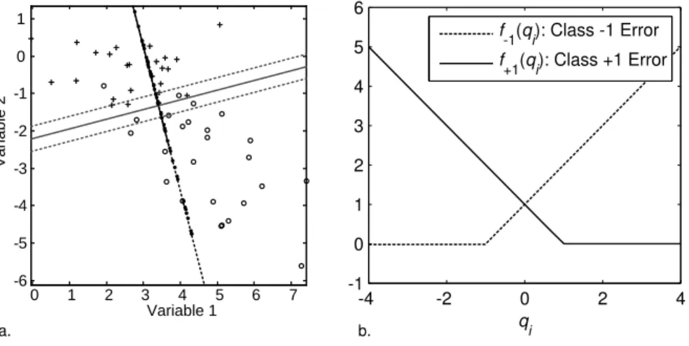
Figure 1: Panel a Projections of the observations in groups 1 (+) and−1 (o) onto the line given by w1 and w2. Panel b shows the absolute hinge error
functionf1(qi) for class 1 objects (solid line) and f−1(qi) for class −1 objects
(dashed line). wherex0
iis rowiofXandcis an intercept. Consider the example in Figure 1a
where for two predictor variables, each rowi is represented by a point labelled ‘+’ for the class 1 and ‘o’ for class−1. Every combination ofw1andw2defines a
direction in this scatter plot. Then, each pointican be projected onto this line. The idea of the SVM is to choose this line in such a way that the projections of the points of class 1 are well separated from those of class −1. The line of separation is orthogonal to the line with projections and the intercept c
determines where exactly it occurs. Note that ifwhas length 1, that is,kwk= (w0w)1/2 = 1, then Figure 1a explains fully the linear combination (1). If w
doesn not have length 1, then the scale values along the projection line should be multiplied bykwk. The dotted lines in Figure 1a show all those points that project to the lines at qi = −1 and qi = 1. These dotted lines are called the
margin lines in SVMs. Note that if there are more than two variables the margin lines become hyperplanes. Summarizing, the SVM has three sets of parameters that determines its solution: (1) the weights normalized to have length 1, that is,w/kwk, (2) the length ofw, that is,kwk, and (3) the interceptc.
SVMs count an error as follows. Every object i from class 1 that projects such thatqi≥1 yields a zero error. However, ifqi<1, then the error is linear
with 1−qi. Similarly, objects in class−1 withqi≤ −1 do not contribute to the
error, but those with qi >−1 contribute linearly withqi+ 1. In other words,
objects that project on the wrong side of their margin contribute to the error, whereas objects that project on the correct side of their margin yield zero error. Figure 1b shows the error functions for the two classes. Because of its hinge form, we call this error function theabsolute hingeerror.
As the length ofw controls how close the margin lines are to each other, it can be beneficial for the number of errors to choose the largestkwkpossible, so that fewer points contribute to the error. To control the kwk, a penalty term that is dependent onkwkis added to the loss function. The penalty term also avoids overfitting of the data.
LetG1andG−1respectively denote the sets of class 1 and−1 objects. Then,
the SVM loss function can be written as
LSVM(c,w) = Pi∈G1max(0,1−qi) + P i∈G−1max(0, qi+ 1) + λw 0w = Pi∈G1f1(qi) + P i∈G−1f−1(qi) + λw 0w
= Class 1 errors + Class−1 errors + Penalty for nonzerow,
(2) where λ >0 determines the strength of the penalty term. For similar
expres-sions, see Hastie, Tibshirani, and Friedman (2001) and Vapnik (2000). Note that (2) can also be expressed as
LSVM(c,w) =
n
X
i=1
max(0,1−yiqi) +λw0w,
which is closer to the expressions used in the SVM literature.
Assume that we have found a c andw that minimizes (2). All the objects
ithat project on the correct side of their margin, contribute with zero error to the loss. As a consequence, these objects could be removed from the analysis without changing the solution. Therefore, all the objects ithat project at the wrong side of their margin and thus induce error or if an object falls exactly on the margin, then these objects determine the solution. Such objects are called support vectors as they form the fundament of the SVM solution. Note that these objects (the support vectors) are not known in advance and, therefore, the analysis needs to be carried out with allnobjects present in the analysis.
What can be seen from (2) is that any error is punished linearly, not quadrat-ically. Thus, SVMs are more robust against outliers than a least-squares loss function. The idea of introducing robustness by absolute errors is not new. For more information on robust multivariate analysis, we refer to Huber (1981), Vapnik (2000), and Rousseeuw and Leroy (2003). In the next section, we discus two other error functions, one of which is robust.
The SVM literature usually presents the SVM loss function as follows (Burges, 1998): LSVMClas(c,w, ξ) = C X i∈G1 ξi+C X i∈G2 ξi+1 2w 0w, (3) subject to 1 + (c+w0xi)≤ξi fori∈G−1 (4) 1−(c+w0x i)≤ξi fori∈G1 (5) ξi ≥0, (6)
whereCis a nonnegative parameter set by the user to weight the importance of the errors represented by the so-called slack variablesξi. Suppose that objecti
inG1projects at the correct side of its margin, that is,qi=c+w0xi≥1. As a
consequence, 1−(c+w0x
i)≤0 so that the correspondingξi can be chosen as
0. Ifiprojects on the wrong side of its margin, thenqi=c+w0xi<1 so that
1−(c+w0x
i)>0. Choosingξi= 1−(c+w0xi) gives the smallestξi satisfying
the restrictions in (4), (5), and (6). As a consequence,ξi= max(0,1−qi) and is
a measure of error. A similar derivation can be made for class−1 objects. Note that in the SVM literature (3) and (6) are often expressed more compactly as
LSVMClas(c,w, ξ) = C n X i=1 ξi+1 2w 0w, subject to yi(c+w0xi)≤1−ξi fori= 1, . . . , n ξi≥0. ChoosingC= (2λ)−1gives LSVMClas(c,w, ξ) = (2λ)−1 X i∈G1 ξi+ X i∈G−1 ξi+ 2λ1 2w 0w = (2λ)−1 X i∈G1 max(0,1−qi) + X i∈G−1 max(0, qi+ 1) +λw0w = (2λ)−1L SVM(c,w).
showing that the two formulations (2) and (3) are exactly the same up to a scaling factor (2λ)−1 and yield the same c and w. However, the advantage of
(2) is that it can be interpreted as a (robust) error function with a penalty. The quadratic penalty term is used for regularization much in the same way as in ridge regression, that is, to force thewj to be close to zero. The penalty is
particularly useful to avoid overfitting. Furthermore, it can be easily seen that
LSVM(c,w) is a convex function in candw because all three terms are convex
incandw. As the function is also bounded below by zero and it is convex, the minimum of LSVM(c,w) is a global one. In fact, (3) allows the problem to be
treated as a quadratic program. However, in Section 5, we optimize (2) directly by the method of iterative majorization.
3
Other Error Functions
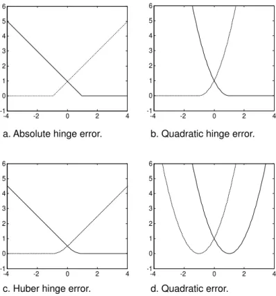
An advantage of clearly separating error from penalty is that it is easy to apply other error functions. Instead of the absolute hinge error in Figure 2a, we can use different definitions for the errorsf1(qi) andf−1(qi). A straightforward
alternative for the absolute hinge error is thequadratic hingeerror, see Figure 2b. This error simply squares the absolute hinge error, yielding the loss function
LQ−SVM(c,w) = X i∈G1 max(0,1−qi)2+ X i∈G−1 max(0, qi+ 1)2+λw0w, (7)
-4 -2 0 2 4 -1 0 1 2 3 4 5 6 -4 -2 0 2 4 -1 0 1 2 3 4 5 6 -4 -2 0 2 4 -1 0 1 2 3 4 5 6 -4 -2 0 2 4 -1 0 1 2 3 4 5 6
a. Absolute hinge error.
c. Huber hinge error.
b. Quadratic hinge error.
d. Quadratic error.
Figure 2: Four error functions: a. the absolute hinge error, b. the quadratic hinge error, c. the Huber hinge error, and d. the quadratic error.
see also,Vapnik (2000) and Cristianini and Shawe-Taylor (2000). It uses the quadratic error for objects that have prediction error and zero error for correctly predicted objects. An advantage of this loss function is that both error and penalty terms are quadratic. In Section 5, we see that the majorizing algorithm is very efficient because in each iteration a linear system is solved very efficiently. A disadvantage of the quadratic hinge error is that outliers can have a large influence on the solution.
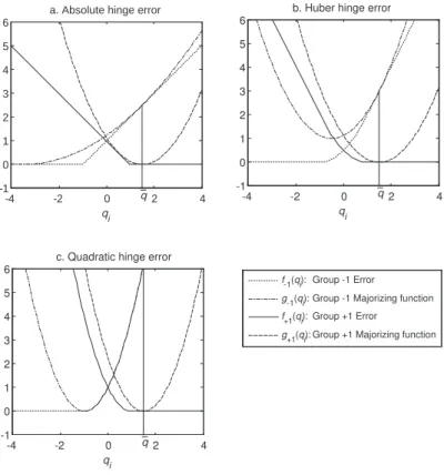
Here, we propose a new smooth and robust alternative: the Huber hinge
error, see Figure 2c. Its definition is found in Table 1 and the corresponding SVM problem is defined by LH−SVM(c,w) = X i∈G1 h+1(qi) + X i∈G−1 h−1(qi) +λw0w. (8)
The Huber hinge error is characterized by a linearly increasing error if the error is large, a smooth quadratic error for errors between 0 and the linear part, and zero for objects that are correctly predicted. The smoothness is governed by a value
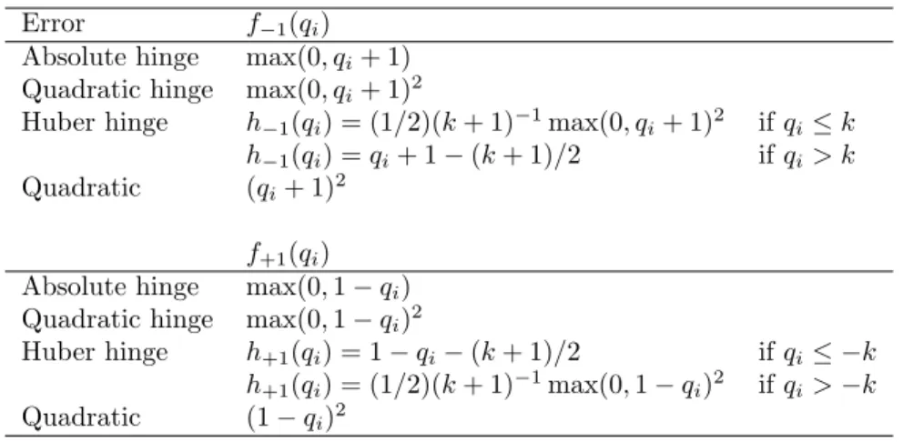
Table 1: Definition of error functions that can be used in the context of SVMs. Error f−1(qi)
Absolute hinge max(0, qi+ 1)
Quadratic hinge max(0, qi+ 1)2
Huber hinge h−1(qi) = (1/2)(k+ 1)−1max(0, qi+ 1)2 ifqi≤k
h−1(qi) =qi+ 1−(k+ 1)/2 ifqi> k
Quadratic (qi+ 1)2
f+1(qi)
Absolute hinge max(0,1−qi)
Quadratic hinge max(0,1−qi)2
Huber hinge h+1(qi) = 1−qi−(k+ 1)/2 ifqi≤ −k
h+1(qi) = (1/2)(k+ 1)−1max(0,1−qi)2 ifqi>−k
Quadratic (1−qi)2
k≥ −1. The Huber hinge approaches the absolute hinge fork↓ −1, so that the Huber hinge SVM loss solution can approach the classical SVM solution. Ifkis chosen too large, then the Huber hinge error essentially approaches the quadratic hinge function. Thus, the Huber hinge error can be seen as a compromise between the absolute and quadratic hinge errors. As we will see in Section 5, it is advantageous to chooseksufficiently large, for example, k= 1, as is done in Figure 2c. A similar computational efficiency as for the quadratic hinge error is also available for the Huber hinge error.
In principle, any robust error can be used. To inherit as much of the nice properties of the standard SVM it is advantageous that the error function has two properties: (1) if the error function is convex inqi (and hence inw), then
the total loss function is also convex and hence has a global minimum that can be reached, (2) the error function should be asymmetric and have the form of a hinge so that objects that are predicted correctly induce zero error.
In Figure 2d the quadratic error is used, defined in Table 1. The quadratic error alone simply equals a multiple regression problem with a dependent vari-ableyi=−1 ifi∈G−1andyi= 1 ifi∈G1, that is,
LMReg(c,w) = X i∈G1 (1−qi)2+ X i∈G−1 (1 +qi)2+λw0w = X i∈G1 (yi−qi)2+ X i∈G−1 (yi−qi)2+λw0w = X i (yi−c−x0iw)2+λw0w = ky−c1−Xwk2+λw0w. (9)
Note that for i ∈ G−1 we have the equality (1 +qi)2 = ((−1)(1 +qi))2 =
Van Gestel, De Brabanter, De Moor, and Vandewalle (2002). To show that (9) is equivalent to ridge regression, we column center X and use JX with
J=I−n−1110 being the centering matrix. Then (9) is equivalent to
LMReg(c,w) = ky−c1−JXwk2n−1110+ky−c1−JXwk2J+λw0w
= ky−c1k2
n−1110+kJy−JXwk2+λw0w, (10)
where the norm notation is defined as kZk2
A = trZ0AZ = Pn i=1 Pn j=1 PK
k=1aijzikzjk. Note that (10) a decomposition in three terms
with the interceptcappearing alone in the first term so that it can be estimated independently of w. The optimal c in (10) equals n−110y. The remaining
optimization of (10) in w simplifies into a standard ridge regression problem. Hence, the SVM with quadratic errors is equivalent to ridge regression. As the quadratic error has no hinge, even properly predicted objects with qi < −1
for i ∈ G−1 or qi > 1 for i ∈ G1 can receive high error. In addition, the
quadratic error is nonrobust, hence can be sensitive to outliers. Therefore, ridge regression is more restrictive than the quadratic hinge error and expected to give worse predictions in general.
4
Optimal Scaling and SVM
Several ideas that are used in SVMs are not entirely new. In this section, we show that the application of optimal scaling known since the 1970s has almost the same aim as the SVM. Optimal scaling in a regression context goes back to the models MONANOVA (Kruskal, 1965), ADDALS (Young, De Leeuw, & Takane, 1976a), MORALS (Young, De Leeuw, & Takane, 1976b), and, more recently, CatREG (Van der Kooij, Meulman, & Heiser, 2006; Van der Kooij, 2007). The main idea of optimal scaling regression (OS-Reg) is that a variabley
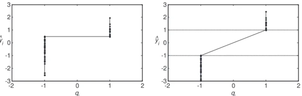
is replaced by an optimally transformed variableyb. The regression loss function is not only optimized over the usual weights, but also over the optimally scaled variable by. Many transformations are possible, see, for example, Gifi (1990). However, to make OS-Reg suitable for the binary classification problem, we use the so-called ordinal transformation with the primary approach to ties. This transformation was proposed in the context of multidimensional scaling to optimally scale the ordinal dissimilarities. As we are dealing with two groups only, this means that the only requirement is to constrain allybi in G−1 to be
smaller than or equal to allybj in G1. An example of such a transformation is
given in Figure 3a.
OS-Reg can be formalized by minimizing
LOS−Reg(by,w) =
n
X
i=1
(byi−x0iw)2+λw0w=kyb−Xwk2+λw0w (11)
subject to byi ≤ybj for all combinations of i∈ G−1 and j ∈ G1 and yb0by =n.
-2 -1 0 1 2 -3 -2 -1 0 1 2 3 q i y i -2 -1 0 1 2 -3 -2 -1 0 1 2 3 q i y ^ i
a. Optimal scaling transformation by primary approach to ties.
b. Optimal scaling transformation for SVMs. ^
Figure 3: Optimal scaling transformationybof the dependent variabley. Panel a shows an example transformation for the OS-Reg, Panel b for SVM.
b
y=0andw=0. In the usual formulation, no penalty term is present in (11), but here we add it because of ease of comparison with SVMs.
The error part of an SVM can also be expressed in terms of an optimally scaled variableby. Then, the SVM loss becomes
LSVM−Abs(by,w, c) =
n
X
i=1
|ybi−x0iw−c|+λw0w (12)
subject toybi≤ −1 ifi∈G−1 and byi≥1 if i∈G1. Clearly, for i∈G−1 a zero
error is obtained ifx0
iw+c≤ −1 by choosingybi =xi0w+c. Ifx0iw+c >−1,
then the restrictionybi ≤ −1 becomes active so that ybi must be chosen as −1.
Similar reasoning holds fori∈G1, whereybi=xi0w+cifx0iw+c≥1 (yielding
zero error) andbyi= 1 ifx0iw+c <1.
Just as the SVM, OS-Reg also has a limited number of support vectors. All objectsithat are below or above the horizontal line yield zero error. All objects
i that are have a value byi that is on the horizontal line generally give error,
hence are support vectors.
The resemblances of SVM and OS-Reg is that both can be used for the binary classification problem, both solutions only use the support vectors, and both can be expressed in terms of an optimal scaled variable by. Although, the SVM estimates the intercept c, OS-Reg implicitly estimates c by leaving the position free where the horizontal line occurs, whereas the SVM attains this freedom by estimatingc. One of the main differences is that OS-Reg uses squared error whereas SVM uses the absolute error. Also, in its standard form
λ= 0 so that OS-Reg does not have a penalty term. A final difference is that OS-Reg solves the degenerate zero loss solution ofyb=0andw=0by imposing the length constraintyb0by=nwhereas the SVM does this through setting having
a minimum difference of 2 betweenbyiandybjifiandjare from different groups.
In some cases withλ= 0, we found occasionally OS-Reg solutions where one of the groups collapsed at the horizontal line and the some objects of the other
group were split into two points: one also at the horizontal line, the other at a distinctly different location. In this way, the length constraint is satisfied, but it is hardly possible to distinguish the groups. Fortunately, these solutions do not occur often and they never occurred with an active penalty term (λ >0).
5
SVM-Maj: A Majorizing Algorithm for SVM
with Robust Hinge Errors
In the SVM literature, the dual of (3) is expressed as a quadratic program and is solved by special quadratic program solvers. A disadvantage of these solvers is that they may become computationally slow for large number of objects n
(although fast specialized solvers exist). Here we derive an iterative majorization (IM) algorithm for the primal SVM problem. An advantage of IM algorithms is that each iteration reduces the SVM loss function. Each of the three loss functions discussed is convex. Because IM is a guaranteed descent algorithm, the IM algorithm will stop when the estimates are sufficiently close to the global minimum. The combination of these properties forms the main strength of the majorization algorithm. In principle, a majorization algorithm can be derived for any error function that has a bounded second derivative as most robust errors have.
Letf(q) be the function to be minimized. Iterative majorization operates on an auxiliary function, called the majorizing functiong(q,q), that is dependent onqand the previous (known) estimateq. The majorizing functiong(q,q) has to fulfill several requirements: (1) it should touchf at the supporting pointy, that is,f(q) =g(q,q), (2) it should never be belowf, that is, f(q)≤g(q,q), and (3)g(q,q) should be simple, preferably linear or quadratic inq. Letq∗ be
such thatg(q∗,q)≤g(q,q), for example, by finding the minimum of g(q,q).
Because the majorizing function is never below the original function, we obtain the so called sandwich inequality
f(q∗)≤g(q∗,q)≤g(q,q) =f(q)
showing that the update q∗ obtained by minimizing the majorizing function
never increases f and usually decreases it. This constitutes a single iteration. By repeating these iterations, a monotonically nonincreasing (usually a decreas-ing) series of loss function valuesf is obtained. For convexf and after a suffi-cient number of iterations, the IM algorithm stops at a global minimum. More information on iterative majorization can be found in De Leeuw (1994), Heiser (1995), Lange, Hunter, and Yang (2000), Kiers (2002), and Hunter and Lange (2004) and an introduction in Borg and Groenen (2005).
An additional property of IM is useful for developing the algorithm. Suppose we have two functions, f1(q) and f2(q), and each of these functions can be
majorized, that is,f1(q) ≤g1(q,q) andf2(q) ≤g1(q,q). Then, the function f(q=f1(q) +f2(q) can be majorized byg(q=g1(q,q) +g2(q,q)
For notational convenience, we refer in the sequel to the majorizing function as
g(q) without the implicit argumentq.
To find an algorithm, we need to find a majorizing function for (2). For the moment, we assume that a quadratic majorizing function exists for each individual error term of the form
f−1(qi) ≤ a−1iq2i −2b−1iqi+c−1i=g−1(qi) (13)
f1(qi) ≤ a1iqi2−2b1iqi+ci=g1(qi). (14)
Then, we combine the results for all terms and come up with the total majorizing function that is quadratic incandwso that an update can be readily derived. In the next subsection, we derive the SVM-Maj algorithm for general hinge errors assuming that (13) and (14) are known for the specific hinge error. In the appendix, we deriveg−1(qi) and g1(qi) for the absolute, quadratic, and Huber
hinge error SVM.
5.1
SVM-Maj
We interpret (2) for use with f−1(q) and f1(q) any of the three hinge errors
discussed above. For deriving the SVM-Maj algorithm, we assume that (13) and (14) are known for these hinge losses. Figure 4 shows that this is the case indeed. Then, let
ai = ½ max(δ, a−1i) ifi∈G−1, max(δ, a1i) ifi∈G1, (15) bi = ½ b−1i ifi∈G−1, b1i ifi∈G1, (16) ci = ½ c−1i ifi∈G−1, c1i ifi∈G1. (17)
Summing all the individual terms leads to the majorization inequality
LSVM(c,w) ≤ n X i=1 aiqi2−2 n X i=1 biqi+ n X i=1 ci+λ m X j=1 w2j. (18)
Becauseqi =c+x0iwi, it is useful to add an extra column of ones as the first
column ofXso thatX becomesn×(m+ 1). Letv0= [cw0] so thatq=Xv.
Now, (2) can be majorized as
LSVM(v) ≤ n X i=1 ai(x0iv)2−2 n X i=1 bix0iv+ n X i=1 ci+λ mX+1 j=2 v2j = v0X0AXv−2v0X0b+c m+λv0Pv = v0(X0AX+λP)v−2v0X0b+c m, (19)
where A is a diagonal matrix with elements ai on the diagonal, bis a vector
with elements bi, andcm =
Pn
f-1(qi): Group -1 Error
g-1(qi): Group -1 Majorizing function f+1(qi): Group +1 Error
g+1(qi): Group +1 Majorizing function
-4 -2 0 2 4 -1 0 1 2 3 4 5 6 qi q a. Absolute hinge error
-4 -2 0 2 4 -1 0 1 2 3 4 5 6 qi q b. Huber hinge error
-4 -2 0 2 4 -1 0 1 2 3 4 5 6 q i q c. Quadratic hinge error
Figure 4: Quadratic majorization functions for (a) the absolute hinge error, (b) the Huber hinge error, and (c) the quadratic hinge error. The supporting point isq= 1.5 both for the Group −1 and 1 error so that the majorizing functions touch atq=q= 1.5.
element p11 = 0. If P wereI, then the last line of (19) would be of the same
form as a ridge regression. Differentiation the last line of (19) with respect to
vyields the system of equalities linear inv
(X0AX+λP)v=X0b. (20)
The update v+ solves this set of linear equalities, for example, by Gaussian
elimination, or, less efficiently, by
v+= (X0AX+λP)−1X0b. (21)
Because of the substitutionv0 = [c w0], the update of the intercept isc+ =v 1
and w+j = v+j+1 for j = 1, . . . , m. The update v+ forms the heart of the
majorization algorithm for SVMs.
Extra computational efficiency can be obtained for the quadratic and Huber hinge errors for whicha−1i=a1i=afor all iand thisadoes not depend onq.
In these cases, (21) simplifies into
v+= (aX0X+λP)−1X0b.
Thus, the m×n matrix S = (aX0X+λP)−1X0 can be computed once and
stored in memory, so that the update (21) simply amounts to settingv+=Sb.
The majorizing algorithm for minimizing the standard SVM in (2) is summa-rized in Algorithm 1. This algorithm has several advantages. First, it iteratively approaches the global minimum closer in each iteration. In contrast, quadratic programming of the dual problem needs to solve the dual problem completely to have the global minimum of the original primal problem. Secondly, the progress can be monitored, for example, in terms of the changes in the number of misclassified objects. Thirdly, to reduce the computational time, smart ini-tial estimates ofcandwcan be given if they are available, for example, from a previous cross validation run. Note that in each majorization iteration a ridge regression problem is solved so that the SVM-Maj algorithm can be seen as a solution to the SVM problem via successive solutions of ridge regressions.
Algorithm:SVM-Maj
input :y,X, λ, ², Hinge
output:ct,wt
t= 0;
Set²to a small positive value;
Setw0 andc0 to random initial values; if Hinge = Huber or Quadratic then
if Hinge = Quadratic thena= 1;
if Hinge = Huber thena= (1/2)(k+ 1)−1; S= (aX0X+λP)−1X0; end ComputeLSVM(c0,w0) according to (2); whilet= 0 or(Lt−1−LSVM(ct,wt))/LSVM(ct,wt)> ²do t=t+ 1; Lt−1=LSVM(ct−1,wt−1);
Comment:Compute A and b for different hinge errors
if Hinge = Absolute then
Computeai by (22) ifi∈G−1 and by (25) ifi∈G1;
Computebi by (23) ifi∈G−1and by (26) ifi∈G1; else if Hinge = Quadratic then
Computebi by (29) ifi∈G−1and by (32) ifi∈G1; else if Hinge = Huber then
Computebi by (35) ifi∈G−1and by (38) ifi∈G1; end
Make the diagonal matrixAwith elements ai;
Comment:Compute update
if Hinge = Absolute then
Findvby that solves (20): (X0AX+λP)v=X0b;
else if Hinge = Huber or Quadratic then v=Sb;
end
Setct=v1andwtj =vj+1 forj = 1, . . . , m; end
Algorithm 1: The SVM majorization algorithm SVM-Maj.
An illustration of the iterative majorization algorithm is given in Figure 5 for the absolute hinge SVM. Here,c is fixed at its optimal value and the mini-mization is only overw, that is, overw1 and w2. Each point in the horizontal
plane represents a combination ofw1 andw2. The majorization function is
in-deed located above the original function and touches it at the dotted line. The
w1 andw2 where this majorization function finds its minimum, LSVM(c,w) is
lower than at the previous estimate, so LSVM(c,w) has decreased. Note that
the separation line and the margins corresponding to the current estimates of
w1 andw2are given together with the class 1 points represented as open circles
Figure 5: Example of the iterative majorization algorithm for SVMs in action wherec is fixed andw1andw2are being optimized. The majorization function
touchesLSVM(c,w) at the previous estimates ofw(the dotted line) and a solid
line is lowered at the minimum of the majorizing function showing a decrease inLSVM(c,w) as well.
6
Experiments
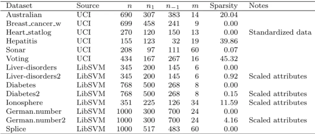
To investigate the performance of the various variants of SVM algorithms, we report experiments on several data sets from the UCI repository (Newman, Hettich, Blake, & Merz, 1998) and the homepage of LibSVM software (Chang & Lin, 2006). These data sets cover a wide range of characteristics such as extent of being unbalanced (one group is larger than the other), number of observationsn, ratio of observations to attributesm/n, and sparsity (the percentage of nonzero attribute valuesxij). More information on the data sets are given in Table 2.
In the experiments, we applied the standard absolute hinge (²-insensitive), the Huber hinge and quadratic hinge SVM loss functions. All experiments have been carried out in Matlab 7.2, on a 2.8Ghz Intel processor with 2GB of memory under Windows XP. The performance of the majorization algorithms is
com-Table 2: Information on the 14 datasets used in the experiments. n1 andn−1
are the number of observations with yi = 1 and yi = −1, respectively.
Spar-sity equals the percentage of zeros in the dataset. The scaling for the scaled attributes is between +1 and 1.
Dataset Source n n1 n−1 m Sparsity Notes
Australian UCI 690 307 383 14 20.04 Breast cancer w UCI 699 458 241 9 0.00
Heart statlog UCI 270 120 150 13 0.00 Standardized data Hepatitis UCI 155 123 32 19 39.86
Sonar UCI 208 97 111 60 0.07
Voting UCI 434 167 267 16 45.32 Liver-disorders LibSVM 345 200 145 6 0.00
Liver-disorders2 LibSVM 345 200 145 6 0.92 Scaled attributes Diabetes LibSVM 768 500 268 8 0.00
Diabetes2 LibSVM 768 500 268 8 0.15 Scaled attributes Ionosphere LibSVM 351 225 126 34 11.59 Scaled attributes German.number LibSVM 1000 300 700 24 0.00
German.number2 LibSVM 1000 300 700 24 4.16 Scaled attributes Splice LibSVM 1000 517 483 60 0.00
pared to those of the off-the-shelf programs LibSVM, BSVM (Hsu & Lin, 2006), SVM-Light (Joachims, 1999), and SVM-Perf (Joachims, 2006). Although these programs can handle nonlinearity of the predictor variables by using special kernels, we limit our experiments to the linear kernel. Note that not all of these SVM-solvers are optimized for the linear kernel. In addition, no comparison between majorization is possible for the Huber hinge loss function as it is not supported by these solvers.
The numerical experiments address several issues. First, how well are the different hinge losses capable of predicting the two groups? Second, we focus on the performance of the majorization algorithm with respect to its competitors. We would like to know how the time needed for the algorithm to converge scales with the number of observationsn, the strictness of the stopping criterion, and withλ; what is a suitable level for the stopping criterion.
To answer these questions, we consider the following measures. First, we define convergence between two steps as the relative decrease in loss between two subsequent steps, that is, byLdiff = (Lt−1−Lt)/Lt. The error rate in the
training data set is defined as the number of misclassified cases. To measure how well a solution predicts, we define the accuracy as the percentage correctly predicted out-of-sample cases in 5-fold cross validation.
6.1
Predictive Performance for the Three Hinge Errors
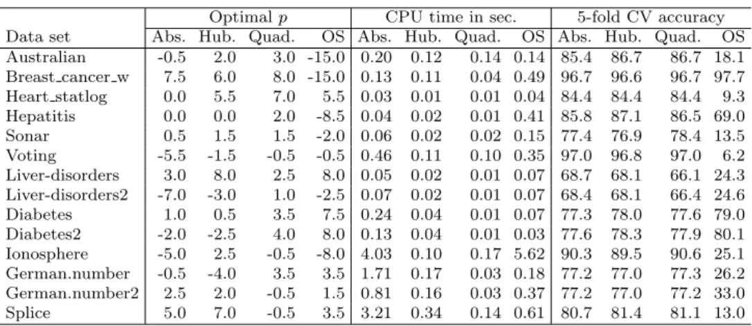
It is interesting to compare the performance of the three hinge loss functions. Consider Table 3, which compares the 5-fold cross-validation accuracy for the three different loss function. For each data set, we tried a grid ofλvalues (λ= 2p
Table 3: Optimal λ = 2p obtained by 5 fold cross validation, the CPU-time
to convergence for the optimal λ, and the prediction accuracy (in %) for 14 different test data sets and four loss functions.
Optimalp CPU time in sec. 5-fold CV accuracy Data set Abs. Hub. Quad. OS Abs. Hub. Quad. OS Abs. Hub. Quad. OS Australian -0.5 2.0 3.0 -15.0 0.20 0.12 0.14 0.14 85.4 86.7 86.7 18.1 Breast cancer w 7.5 6.0 8.0 -15.0 0.13 0.11 0.04 0.49 96.7 96.6 96.7 97.7 Heart statlog 0.0 5.5 7.0 5.5 0.03 0.01 0.01 0.04 84.4 84.4 84.4 9.3 Hepatitis 0.0 0.0 2.0 -8.5 0.04 0.02 0.01 0.41 85.8 87.1 86.5 69.0 Sonar 0.5 1.5 1.5 -2.0 0.06 0.02 0.02 0.15 77.4 76.9 78.4 13.5 Voting -5.5 -1.5 -0.5 -0.5 0.46 0.11 0.10 0.35 97.0 96.8 97.0 6.2 Liver-disorders 3.0 8.0 2.5 8.0 0.05 0.02 0.01 0.07 68.7 68.1 66.1 24.3 Liver-disorders2 -7.0 -3.0 1.0 -2.5 0.07 0.02 0.01 0.07 68.4 68.1 66.4 24.6 Diabetes 1.0 0.5 3.5 7.5 0.24 0.04 0.01 0.07 77.3 78.0 77.6 79.0 Diabetes2 -2.0 -2.5 4.0 8.0 0.13 0.04 0.01 0.03 77.6 78.3 77.9 80.1 Ionosphere -5.0 2.5 -0.5 -8.0 4.03 0.10 0.17 5.62 90.3 89.5 90.6 25.1 German.number -0.5 -4.0 3.5 3.5 1.71 0.17 0.03 0.18 77.2 77.0 77.3 26.2 German.number2 2.5 2.0 -0.5 1.5 0.81 0.16 0.03 0.37 77.2 77.0 77.2 33.0 Splice 5.0 7.0 -0.5 3.5 3.21 0.34 0.14 0.61 80.7 81.4 81.1 13.0
Alongside are given the values of the optimalλ’s and times to convergence (stop wheneverLdiff <3×10⁻⁷). From the accuracy, we see that there is no one best
loss function that is suitable for all data sets. The absolute hinge is best in six of the cases, the Huber hinge is best in six of the cases, and the quadratic hinge is best in eight of the cases. The total number is greater than 14 due to equal accuracies. In terms of computational speed, the order invariably is: absolute hinge is the slowest, Huber hinge is faster, and the quadratic hinge is the fastest. The implementation of optimal scaling regression was also done in MatLab, but the update in each iteration forbyby monotone regression using the primary approach to ties was calculated by a compiled Fortran subroutine. Therefore, the CPU time is not comparable to those of the other SVM methods that were solely programmed in MatLab. Optimal scaling regression performs well on three data sets (Breast cancer, Diabetes and Diabetes2) where the accuracy is better than the three SVM methods. On the remaining data sets, the accuracy is worse or much worse when compared to the SVM methods. It seems that in some cases OS regression can predict well, but its poor performance for the majority of the data sets makes it hard to use it as a standard method for the binary classification problem. It seems that more study is needed to understand why this is so and, if possible, provide adaptations that make it work better for more data sets.
6.2
Computational Efficiency of SVM-Maj
To see how computationally efficient the majorization algorithms are, two types of experiments were done. In the first experiment, the majorization algorithm
is studied and tuned. In the second, the majorization algorithm SVM-Maj for the absolute hinge error is compared with several off-the-shelf programs that minimize the same loss function.
As the majorization algorithm is guaranteed to improve the LSVM(c,w) in
each iteration by taking a step closer to the final solution, the computational efficiency of SVM-Maj is determined by its stopping criterion. The iterations of SVM-Maj stop wheneverLdiff < ². It is also known that majorization algorithms
have a linear convergence rate (De Leeuw, 1994), which can be slow especially for very small ². Therefore, we study the relations between four measures as they change during the iterations: (a) the difference between present and final loss,Lt−Lfinal, (b) the convergenceLdiff, (c) CPU time spent sofar, and (d)
the difference between current and final within sample error rate.
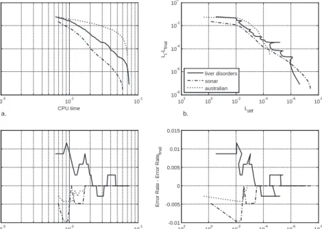
Figure 6 shows the relationships between these measures for three exemplary data sets: Liver disorders, Sonar and Australian. Note that Figures 6c and 6d the direction of the horizontal axis is reversed so that in all four panels the right side of the horizontal axis means more computational investment. Figure 6a draws the relationship between CPU-time on the one hand andLt−Lfinal, with Lfinalthe objective function values obtained at convergence with ²= 3×10⁻⁷.
Notice that in most of the cases the first few iterations are responsible for the bulk of the decreases in the objective function values and most of the CPU time is spent to obtain small decreases in loss function values. Figure 6b shows the relationship betweenLt−Lfinal and the convergenceLdiff that is used as a
stopping criterion. The two lower panels show the development of the within sample error rate and CPU time (Figure 6c) and convergenceLdiff (Figure 6d).
To evaluate whether it is worthwhile using a looser stopping criterion, it is in instructive to observe the path of the error rate over the iterations (the lower right panel). It seems that the error rate stabilizes for values ofLdiffbelow 10−6.
Nevertheless, late-time changes sometimes occur in other data sets. Therefore, it does not seem recommendable to stop the algorithm much earlier, hence our recommendation of using²= 3×10⁻⁷.
The analogues of Figures 6 and 7 were also produced for the Huber hinge and quadratic hinge loss functions. Overall, the same patterns as for the abso-lute hinge function can be distinguished, with several differences: the objective function decreases much faster (relative to CPU time), and the error rate stabi-lizes already at slightly greater values for the convergence criterion. In addition, the number of iterations until convergence by and large decline (vis-a-vis the absolute hinge function).
Figure 7 investigates how sensitive the speed of SVM-Maj is relative to changes in the values ofλfor four illustrative datasets (Splice, German-number with scaled attributed, Ionosphere, and Sonar). As expected, the relationship appears to be decreasing. Thus, for largeλthe penalty term dominatesLSV M
and the SVMMajAbs does not need too many iterations to converge. Note that the same phenomenon is in general observed for the other SVM-solvers as well so that, apparently, the case for largeλis an easier problem to solve.
10-3 10-2 10-1 10-8 10-6 10-4 10-2 100 CPU time Lt -Lfina l 10-8 10-6 10-4 10-2 100 102 10-8 10-6 10-4 10-2 100 Ldiff Lt -Lfina l 10-3 10-2 10-1 -0.01 -0.005 0 0.005 0.01 0.015 CPU time Error R at e - Er ror R ate fi n al 10-8 10-6 10-4 10-2 100 102 -0.01 -0.005 0 0.005 0.01 0.015 Ldiff Error R at e - Er ror R ate fi n al liver disorders sonar australian a. b. c. d.
Figure 6: The evolution of several statistics (see text for details) of three datasets: Australian (dotted lines), Sonar (dash-dot lines), and Liver Disorders (scaled, solid lines). Values ofλ’s are fixed at optimal levels for each dataset. Loss function used: absolute hinge.
6.3
Comparing Efficiency of SVM-Maj with Absolute Hinge
The efficiency of SVM-Maj can be compared with off-the-shelf programs for the absolute hinge error. As competitors of SVM-Maj, we use LibSVM, BSVM, SVM-Light, and SVM-Perf. We use the same 14 data sets as before. As all methods minimize exactly the same loss functionLSVMthey all should have the
same global minimum. In addition toLSVM, the methods are compared on speed
(CPU-time in seconds) at optimal levels of theλ= 2p(or equivalent) parameter.
Note that the optimal levels ofλ could differ slightly between methods as the off-the-shelf programs perform their own grid search for determining the optimal
λ, that could be slightly different from those reported in Table 3. We note that the relationship between theλparameter in SVM-Maj and theC parameter in LibSVM and SVM-light is given byλ= 0.5/C. For SVM-Maj, we choose three stopping criteria, that is, the algorithm is stopped wheneverLdiffis respectively
smaller than 10−4,10−5, and 10−6.
For some data sets, it was not possible to run the off-the-shelf programs, sometimes because the memory requirements were too large, sometimes be-cause no convergence was obtained. Such problems occurred for three data sets
−15 −10 −5 0 5 10 −1.5 −1 −0.5 0 0.5 1 log2(Lambda) log10(CPU time) Splice German.number2 Ionosphere Sonar
Figure 7: The effect of changingλon CPU time taken to converge. Loss function used: absolute hinge.
with SVM-Perf and two data sets with SVM-Light. Table 4 shows the results. Especially for ² = 10−6, SVM-Maj gives solutions that are close to the best
minimum found. Generally, Lib-SVM and SVM-Light obtain the lowestLSVM.
SVM-Maj performs well with²= 10−6, but even better values can be obtained
by a stronger convergence criterion. BSVM finds proper minima but is not able to handle all data sets. In terms of speed SVM-Maj is faster than its com-petitors in almost all cases. Of course, a smaller² increases the CPU-time of SVM-Maj. Nevertheless, even for ²= .0001 good solutions can be found in a short CPU-time.
These results are also summarized in Figure 8, where SVM-Maj is used with the default convergence criterion of²= 3×10⁻⁷. As far as speed is concerned
(see Figure 8a), SVM-Maj ranks consistently amongst the fastest method. The quality of SVM-Maj is also consistently good as it has the same loss function as the global minimum with differences occurring less then 0.01. Note that BSVM and SVM-Perf find consistently much higher loss function values than SVM-Maj, LibSVM and SVM-Light. Generally, the best quality solutions are obtained by LibSVM and SVM-Light although they tend to use more CPU time reaching it.
7
Conclusions and Discussion
We have discussed how linear SVM can be viewed as a the minimization of a robust error function with a regularization penalty. The regularization is needed to avoid overfitting in the case when the number of predictor variables increases. We provided a new majorization algorithm for the minimization of the primal SVM problem. This algorithm handles the standard absolute hinge error, the quadratic hinge error, and the newly proposed Huber hinge
10-2 100 102 104 Splice German.number2 German.number Ionosphere Diabetes2 Diabetes Liver-disorders2 Liver-disorders Voting Sonar Hepatitis Heart_statlog Breast_cancer_w Australian
CPU time in sec
10-10 10-5 100 105 Splice German.number2 German.number Ionosphere Diabetes2 Diabetes Liver-disorders2 Liver-disorders Voting Sonar Hepatitis Heart_statlog Breast_cancer_w Australian L - Llowest SVM-Maj LibSVM BSVM SVM-Light SVM-Perf a. b.
Figure 8: Difference in performance of SVM algorithms with absolute hinge and SVM-Maj using² = 3×10⁻⁷. Panel a shows the CPU time used in seconds
and Panel b shows the difference ofLand the lowestLamongst the methods. error. The latter hinge is smooth everywhere yet is linear for large errors. The majorizing algorithm has the advantage that it operates on the primal, is easy to program, and can easily be adapted for robust hinge errors. We also showed that optimal scaling regression has several features in common with SVMs. Numerical experiments on fourteen empirical data sets showed that there is no clear difference between the three hinge errors in terms of cross validated accuracy. The speed of SVM-Maj for the absolute hinge error is similar or compares favorably to the off-the-shelf programs for solving linear SVMs.
There are several open issues and possible extensions. First, the SVM-Maj algorithm is good for situations where the number of objectsnis (much) larger than the number of variables m. The reason is that each iteration solves an (m+ 1)×(m+ 1) linear system. As mgrows, each iteration becomes slower. Other majorization inequalities can be used to solve this problem yielding fast iterations at the cost of making (much) smaller steps in each iteration. A second limitation is the size ofn. Eventually, whenngets large, than iterations will be-come slow. The good thing about SVM-Abs is that each iteration is guaranteed to improve the SVM-Loss. The bad thing is that at most linear convergence can be reached so that for largen one has to be satisfied with an approximate
solution only.
Second, this paper has focussed on linear SVMs. Nonlinearity can be brought in in two ways. In (Groenen et al., 2007), we proposed to use optimal scaling for the transformation of the predictor variables. Instead of using kernels, we propose to use I-splines to accommodate nonlinearity in the predictor space. The advantage of this approach is that it can be readily applied in any linear SVM algorithm. The standard way of introducing nonlinearity in SVMs is by using kernels. We believe that this is also possible for SVM-Maj and intend to study this possibility in future publications.
SVMs can be extended to problems with more than two classes in several ways. If the extension has error terms of the form f1(q) or f−1(q) then the
present majorization results can be readily applied for an algorithm. We be-lieve that applying majorization to SVMs is a fruitful idea that opens new applications and extensions to this area of research.
References
Borg, I., & Groenen, P. J. F. (2005). Modern multidimensional scaling: Theory and applications (2nd edition). New York: Springer.
Burges, C. J. C. (1998). A tutorial on support vector machines for pattern recognition. Knowledge Discovery and Data Mining, 2, 121–167.
Chang, C.-C., & Lin, C.-J. (2006). LIBSVM: a library for support vector machines.(Software available athttp://www.csie.ntu.edu.tw/~cjlin/ libsvm)
Cristianini, N., & Shawe-Taylor, J. (2000). An introduction to support vector machines. Cambridge University Press.
De Leeuw, J. (1994). Block relaxation algorithms in statistics. In H.-H. Bock, W. Lenski, & M. M. Richter (Eds.),Information systems and data analysis
(pp. 308–324). Berlin: Springer.
Gifi, A. (1990). Nonlinear multivariate analysis. Chichester: Wiley.
Groenen, P. J. F., Nalbantov, G., & Bioch, J. C. (2007). Nonlinear support vector machines through iterative majorization. In R. Decker & H.-J. Lenz (Eds.),Advances in data analysis (pp. 149–162). Berlin: Springer. Hastie, T., Tibshirani, R., & Friedman, J. (2001). The elements of statistical
learning. New York: Springer.
Heiser, W. J. (1995). Convergent computation by iterative majorization: Theory and applications in multidimensional data analysis. In W. J. Krzanowski (Ed.),Recent advances in descriptive multivariate analysis (pp. 157–189). Oxford: Oxford University Press.
Hsu, C.-W., & Lin, C.-J. (2006). BSVM: bound-constrained support vector machines.(Software available athttp://www.csie.ntu.edu.tw/~cjlin/ bsvm/index.html)
Huber, P. J. (1981). Robust statistics. New York: Wiley.
Hunter, D. R., & Lange, K. (2004). A tutorial on MM algorithms.The American Statistician,39, 30–37.
Joachims, T. (1999). Making large-scale SVM learning practical. In B. Sch¨olkopf, C. Burges, & A. Smola (Eds.),Advances in kernel methods -support vector learning.MIT-Press. (http://www-ai.cs.uni-dortmund. de/DOKUMENTE/joachims_99a.pdf)
Joachims, T. (2006). Training linear SVMs in linear time. InProceedings of the ACM conference on knowledge discovery and data mining (KDD). (http: //www.cs.cornell.edu/People/tj/publications/joachims_06a.pdf) Kiers, H. A. L. (2002). Setting up alternating least squares and iterative ma-jorization algorithms for solving various matrix optimization problems.
Computational Statistics and Data Analysis,41, 157–170.
Kruskal, J. B. (1965). The analysis of factorial experiments by estimating monotone transformations of the data. Journal of the Royal Statistical Society, Series B,27, 251–263.
Lange, K., Hunter, D. R., & Yang, I. (2000). Optimization transfer using surrogate objective functions. Journal of Computational and Graphical Statistics,9, 1–20.
Newman, D., Hettich, S., Blake, C., & Merz, C. (1998). UCI repository of machine learning databases. (http://www.ics.uci.edu/~mlearn/ MLRepository.htmlUniversity of California, Irvine, Dept. of Information and Computer Sciences)
Rousseeuw, P. J., & Leroy, A. M. (2003).Robust regression and outlier detection.
New York: Wiley.
Suykens, J. A. K., Van Gestel, T., De Brabanter, J., De Moor, B., & Vandewalle, J. (2002). Least squares support vector machines. Singapore: World Scientific.
Van der Kooij, A. J. (2007). Prediction accuracy and stability of regression with optimal scaling transformations. Unpublished doctoral dissertation, Leiden University.
Van der Kooij, A. J., Meulman, J. J., & Heiser, W. J. (2006). Local minima in Categorical Multiple Regression. Computational Statistics and Data Analysis,50, 446–462.
Vapnik, V. N. (2000). The nature of statistical learning theory. New York: Springer.
Young, F. W. (1981). Quantitative analysis of qualitative data.Psychometrika,
46, 357–388.
Young, F. W., De Leeuw, J., & Takane, Y. (1976a). Additive structure in qualitative data: An alternating least squares method with optimal scaling features. Psychometrika,41, 471–503.
Young, F. W., De Leeuw, J., & Takane, Y. (1976b). Regression with qualita-tive and quantitaqualita-tive variables: An alternating least squares method with optimal scaling features. Psychometrika,41, 505–529.
A
Majorizing the Hinge Errors
Here we derive the quadratic majorizing functions for the three hinge functions.
A.1
Majorizing the Absolute Hinge Error
Consider the termf−1(q) = max(0, q+ 1). For notational convenience, we drop
the subscripti for the moment. The solid line in Figure 2a showsf−1(q).
Be-cause of its shape of a hinge, we have called this function the absolute hinge function. Letqbe the known errorqof the previous iteration. Then, a majoriz-ing function forf−1(q) is given byg−1(q, q) at the supporting pointq= 2. We
wantg−1(q) to be quadratic so that it is of the formg−1(q) =a−1q2−2b−1q+c−1.
To find a−1, b−1, andc−1, we impose two supporting points, one atq and the
other at−2−q. These two supporting points are located symmetrically around
−1. Note that the hinge function is linear at both supporting points, albeit with different gradients. Becauseg−1(q) is quadratic, the additional requirement that f−1(q)≤g−1(q) is satisfied ifa−1>0 and the derivatives at the two supporting
points off−1(q) andg−1(q) are the same. More formally, the requirements are
that f−1(q) = g−1(q), f0 −1(q) = g−0 1(q), f−1(−2−q) = g−1(−2−q), f0 −1(−2−q) = g−0 1(−2−q), f−1(q) ≤ g−1(q).
It can be verified that the choice of
a−1 = 14|q+ 1|−1, (22)
b−1 = −a−1−14, (23)
c−1 = a−1+21+14|q+ 1|, (24)
satisfies all these requirements. Figure 4a shows the majorizing functiong−1(q)
For Class 1, a similar majorizing function can be found forf1(q) = max(0,1− q). However, in this case, we require equal function values and first derivative atqand at 2−q, that is, symmetric around 1. The requirements are
f1(q) = g1(q), f0 1(q) = g10(q), f1(2−q) = g1(2−q), f0 1(2−q) = g10(2−q), f1(q) ≤ g1(q). Choosing a1 = 14|1−q|−1 (25) b1 = a1+14 (26) c1 = a1+12+14|1−q| (27)
satisfies these requirements. The functions f1(q) and g1(q) with supporting
pointsq= 2 orq= 0 are plotted in Figure 4a.
Note thata−1is not defined ifq=−1. In that case, we choosea−1as a small
positive constantδthat is smaller than the convergence criterion²(introduced below). Strictly speaking, the majorization requirements are violated. How-ever, by choosingδsmall enough, the monotone convergence of the sequence of
LSVM(w) will be no problem. The same holds fora1 ifq= 1.
A.2
Majorizing the Quadratic Hinge Error
The majorizing algorithm for the SVM with the quadratic hinge function is developed along the same lines as for the absolute hinge function. However, because of its structure, each iteration boils down to a matrix multiplication of an fixedm×n matrix with an n×1 vector that changes over the iterations. Therefore, the computation of the update is of order O(nm) which is more efficient than the majorizing algorithm for the absolute hinge error.
To majorize the termf−1(q) = max(0, q+ 1)2is relatively easy. Forq >−1, f−1(q) coincides with (q+ 1)2. Therefore, if q > −1, (q+ 1)2 can be used to
majorize max(0, q+ 1)2. Note that (q+ 1)2≥0 so that (q+ 1)2also satisfies the
majorizing requirements forq <1. For the case q≤ −1, we want a majorizing function that has the same curvature as (q+ 1)2 but touches at q, which is
obtained by the majorizing function (q+ 1−(q+ 1))2 = (q−q)2. Therefore,
the majorizing functiong−1=a−1q2−2b−1q+c−1has coefficients
a−1 = 1, (28) b−1 = ½ q ifq≤ −1 −1 ifq >−1 , (29) c−1 = ½ 1−2(q+ 1) + (q+ 1)2 ifq≤ −1 1 ifq >−1 . (30)
Similar reasoning can be held forf1(q) = max(0,1−q)2 which has majorizing
functiong1=a1q2−2b1q+c1 and coefficients
a1 = 1, (31) b1 = ½ 1 ifq≤1 q ifq >1 , (32) c1 = ½ 1 ifq≤1 1−2(1−q) + (1−q)2 ifq >1 . (33)
Again,ai, bi,andci are defined as in (15), (16), and (17), except thatδin (15)
can be set to 0, so thatai= 1 =afor alli.
A.3
Majorizing the Huber Hinge Error
The majorizing algorithm of the Huber hinge error function shares a similar efficiency as for the quadratic hinge: the coefficientsa1 and a−1 are the same
for all i, so that again an update boils down to a matrix multiplication of a matrix of orderm×nwith ann×1 vector.
To majorize h−1(q) we use the fact that the second derivative of h−1(q)
is bounded. For q ≥ k, h−1(q) is linear with first derivative h0−1(q) = 1, so
that its second derivative h00
−1(q) = 0. For q ≤ −1, h−1(q) = 0, so that here
too h00
−1(q) = 0. Therefore, h00−1(q) > 0 only exists for −1 < q < k, where h00
−1(q) = 1. Therefore, for −1 < q < k, the quadratic majorizing function is
equal toh−1(q), for q ≤ −1 and q ≥k, a quadratic majorizing function with
the same second derivative of (1/2)(k+ 1)−1 is produced that touches at the
current estimateq. Let the majorizing functiong−1=a−1q2−2b−1q+c−1 has
coefficients a−1 = (1/2)(k+ 1)−1, (34) b−1 = a−1q ifq≤ −1 −a−1 if −1< q < k a−1q−1/2 ifq≥k , (35) c−1 = a−1q2 ifq≤ −1 a−1 if −1< q < k 1−(k+ 1)/2 +a−1q2 ifq≥ −k . (36)
It may be verified for anyqfrom the three intervals thath−1(q) =g−1(q) and h0
−1(q) = g0−1(q) hold. In addition,g00−1(q) = (1/2)(k+ 1)−1 ≥h00−1(q) for all q (as long as k > −1) so that the second derivative d00
−1(q) of the difference
functiond−1(q) =g−1(q)−h−1(q) equalsg00−1(q)−h00−1(q)≥0 indicating that d−1(q) is convex. Asg−1(q) touchesh−1(q) atq,d−1(q) = 0, so that, combined
with convexity of d−1(q) the inequality d−1(q) ≥ 0 must hold implying the
majorizing inequalityh−1(q)≤g−1(q) for allq with equality atq.
For h1(q) similar reasoning can be held. Let the majorizing functiong1 = a−1q2−2b−1q+c−1 has coefficients
b1 = 1/2 +a1q ifq≤ −k a1 if −k < q <1 a1q ifq≥1 , (38) c1 = 1−(k+ 1)/2 +a−1q2 ifq≤ −k a1 if −k < q <1 a1q2 ifq≥1 . (39)
Note that a−1 and a1 are exactly the same and both independent of q.
Therefore, the curvature of the majorizing functions for all Huber hinge errors is the same. This property is exploited in the simple update derived from (22).
Table 4: Comparisons between SVM solvers: time to convergence in CPU sec. and objective values. The values of λ = 2p’s are fixed at levels close to the
optimal ones of Table 3.
Time to con v erge, in CPU sec. LSVM SVMMa j Lib- SVM-SVMMa j Lib- SVM-Dataset p 10 − 4 10 − 5 10 − 6 SVM BSVM Ligh t P erf 10 − 4 10 − 5 10 − 6 SVM BSVM Ligh t P erf Australian 0 0.07 0.08 0.11 6395.27 0.30 76.80 – 202.67 202.69 202.66 207.32 220.81 202.20 – Breast cancer w 6 0.03 0.06 0.10 0.06 0.18 0.09 0.89 58.21 58.05 58.02 58.03 205.03 58.03 205.02 Heart statlog 0 0.02 0.02 0.02 0.08 0.14 0.10 1.43 91.50 91.49 91.49 91.48 91.52 91.48 91.52 Hepatitis 0 0.01 0.02 0.03 0.05 0.09 0.06 62.14 46.31 46.29 46.28 46.28 48.43 46.28 48.43 Sonar 0 0.02 0.04 0.05 0.13 0.30 0.15 31.08 114.54 114.51 114.51 114.51 116.83 114.51 116.83 V oting -5 0.06 0.11 0.11 0.09 0.13 0.12 5.15 26.46 25.76 25.76 25.76 25.76 25.76 25.76 Liv er-disorders 3 0.04 0.06 0.06 0.49 1.25 – – 248.56 248.43 248.42 248.42 253.03 – – Liv er-disorders2 -6 0.03 0.04 0.07 0.11 0.15 – – 249.67 249.62 249.59 249.59 249.63 – – Diab etes 1 0.06 0.09 0.15 33.05 1.88 10.30 407.81 396.73 396.60 396.57 396.81 444.18 396.57 444.18 Diab etes2 -2 0.05 0.07 0.12 0.14 0.23 0.26 77.35 399.81 399.69 399.66 399.66 399.67 399.66 399.66 Ionosphere -5 0.12 0.15 0.38 0.24 0.67 0.88 233.19 55.63 55.51 55.33 55.32 56.56 55.32 56.56 German.n um b er 0 0.13 0.35 0.55 15.21 0.54 1.87 87.73 522.37 521.94 521.89 521.88 524.33 521.88 524.33 German.n um b er2 3 0.14 0.22 0.38 0.27 0.39 0.23 82.49 539.51 539.44 539.40 539.39 539.63 539.39 539.63 Splice 5 0.55 1.01 1.55 0.47 0.87 0.33 11.50 427.37 427.21 427.19 427.18 433.68 427.18 433.68