The Application of Hidden Markov Models in Speech Recognition

Foundations and TrendsR in Signal Processing

Vol. 1, No. 3 (2007) 195–304 c

2008 M. Gales and S. Young DOI: 10.1561/2000000004

The Application of Hidden Markov Models

in Speech Recognition

Mark Gales

and Steve Young

1 _{Cambridge University Engineering Department, Trumpington Street,}

Cambridge, CB2 1PZ, UK, [email protected]

2 _{Cambridge University Engineering Department, Trumpington Street,}

Cambridge, CB2 1PZ, UK, [email protected]

Abstract

Hidden Markov Models (HMMs) provide a simple and effective frame-work for modelling time-varying spectral vector sequences. As a con-sequence, almost all present day large vocabulary continuous speech recognition (LVCSR) systems are based on HMMs.

Whereas the basic principles underlying HMM-based LVCSR are rather straightforward, the approximations and simplifying assump-tions involved in a direct implementation of these principles would result in a system which has poor accuracy and unacceptable sen-sitivity to changes in operating environment. Thus, the practi-cal application of HMMs in modern systems involves considerable sophistication.

The aim of this review is first to present the core architecture of a HMM-based LVCSR system and then describe the various refine-ments which are needed to achieve state-of-the-art performance. These

discriminative parameter estimation, adaptation and normalisation, noise compensation and multi-pass system combination. The review concludes with a case study of LVCSR for Broadcast News and Conversation transcription in order to illustrate the techniques described.

1

Introduction

Automatic continuous speech recognition (CSR) has many potential applications including command and control, dictation, transcription of recorded speech, searching audio documents and interactive spoken dialogues. The core of all speech recognition systems consists of a set of statistical models representing the various sounds of the language to be recognised. Since speech has temporal structure and can be encoded as a sequence of spectral vectors spanning the audio frequency range, the hidden Markov model (HMM) provides a natural framework for constructing such models [13].

HMMs lie at the heart of virtually all modern speech recognition systems and although the basic framework has not changed significantly in the last decade or more, the detailed modelling techniques developed within this framework have evolved to a state of considerable sophisti-cation (e.g. [40, 117, 163]). The result has been steady and significant progress and it is the aim of this review to describe the main techniques by which this has been achieved.

The foundations of modern HMM-based continuous speech recog-nition technology were laid down in the 1970’s by groups at Carnegie-Mellon and IBM who introduced the use of discrete density HMMs

[11, 77, 108], and then later at Bell Labs [80, 81, 99] where

continu-ous density HMMs were introduced.1 An excellent tutorial covering the

basic HMM technologies developed in this period is given in [141]. Reflecting the computational power of the time, initial develop-ment in the 1980’s focussed on either discrete word speaker dependent large vocabulary systems (e.g. [78]) or whole word small vocabulary speaker independent applications (e.g. [142]). In the early 90’s, atten-tion switched to continuous speaker-independent recogniatten-tion.

Start-ing with the artificial 1000 word Resource Management task [140],

the technology developed rapidly and by the mid-1990’s, reasonable accuracy was being achieved for unrestricted speaker independent dic-tation. Much of this development was driven by a series of DARPA and NSA programmes [188] which set ever more challenging tasks culminating most recently in systems for multilingual transcription of broadcast news programmes [134] and for spontaneous telephone conversations [62].

Many research groups have contributed to this progress, and each will typically have its own architectural perspective. For the sake of log-ical coherence, the presentation given here is somewhat biassed towards the architecture developed at Cambridge University and supported by

the HTK Software Toolkit [189].2

The review is organised as follows. Firstly, in Architecture of a

HMM-Based Recogniser the key architectural ideas of a typical HMM-based recogniser are described. The intention here is to present an over-all system design using very basic acoustic models. In particular, simple single Gaussian diagonal covariance HMMs are assumed. The following

sectionHMM Structure Refinements then describes the various ways in

which the limitations of these basic HMMs can be overcome, for exam-ple by transforming features and using more comexam-plex HMM output distributions. A key benefit of the statistical approach to speech recog-nition is that the required models are trained automatically on data.

1_{This very brief historical perspective is far from complete and out of necessity omits many} other important contributions to the early years of HMM-based speech recognition. 2_{Available for free download athtk.eng.cam.ac.uk. This includes a recipe for building a}

state-of-the-art recogniser for the Resource Management task which illustrates a number of the approaches described in this review.

199

The section Parameter Estimation discusses the different objective

functions that can be optimised in training and their effects on perfor-mance. Any system designed to work reliably in real-world applications must be robust to changes in speaker and the environment. The section on Adaptation and Normalisation presents a variety of generic

tech-niques for achieving robustness. The following section Noise

Robust-nessthen discusses more specialised techniques for specifically handling

additive and convolutional noise. The section Multi-Pass Recognition

Architectures returns to the topic of the overall system architecture and explains how multiple passes over the speech signal using differ-ent model combinations can be exploited to further improve perfor-mance. This final section also describes some actual systems built for transcribing English, Mandarin and Arabic in order to illustrate the various techniques discussed in the review. The review concludes in

2

Architecture of an HMM-Based Recogniser

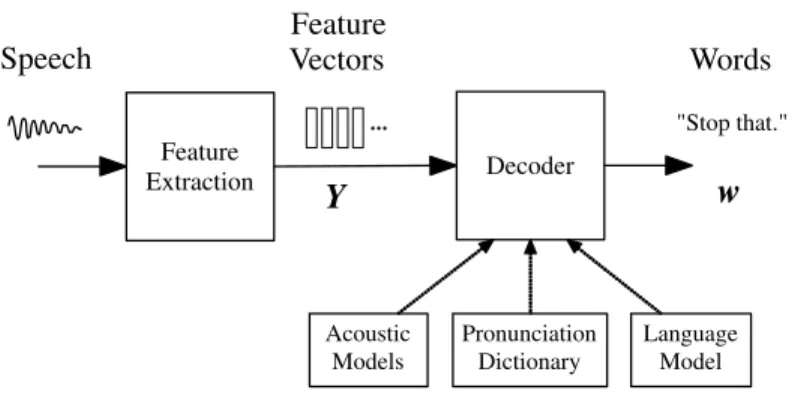
The principal components of a large vocabulary continuous speech recogniser are illustrated in Figure 2.1. The input audio waveform from a microphone is converted into a sequence of fixed size acoustic vectors Y1:T =y1, . . . ,yT in a process called feature extraction. The decoder

then attempts to find the sequence of words w1:L=w1, . . . , wL which

is most likely to have generatedY, i.e. the decoder tries to find ˆ

w= arg max

w {P(w|Y)}. (2.1)

However, since P(w|Y) is difficult to model directly,1 Bayes’ Rule is used to transform (2.1) into the equivalent problem of finding:

ˆ

w= arg max

w {p(Y|w)P(w)}. (2.2)

The likelihood p(Y|w) is determined by an acoustic model and the

priorP(w) is determined by alanguage model.2 The basic unit of sound 1_{There are some systems that are based on discriminative models [54] whereP(w|Y) is} modelled directly, rather than using generative models, such as HMMs, where the obser-vation sequence is modelled,p(Y|w).

2_{In practice, the acoustic model is not normalised and the language model is often scaled} by an empirically determined constant and a word insertion penalty is added i.e., in the log domain the total likelihood is calculated as logp(Y|w) +αlog(P(w)) +β|w|whereα is typically in the range 8–20 andβis typically in the range 0 –−20.

2.1 Feature Extraction 201 Feature Extraction Decoder Y w Speech Feature Vectors Words "Stop that." Acoustic Models Pronunciation Dictionary Language Model ...

Fig. 2.1 Architecture of a HMM-based Recogniser.

represented by the acoustic model is thephone. For example, the word

“bat” is composed of three phones /b/ /ae/ /t/. About 40 such phones are required for English.

For any given w, the corresponding acoustic model is

synthe-sised by concatenating phone models to make words as defined by a pronunciation dictionary. The parameters of these phone models are estimated from training data consisting of speech waveforms and their orthographic transcriptions. The language model is typically

an N-gram model in which the probability of each word is

condi-tioned only on its N −1 predecessors. The N-gram parameters are

estimated by counting N-tuples in appropriate text corpora. The

decoder operates by searching through all possible word sequences using pruning to remove unlikely hypotheses thereby keeping the search tractable. When the end of the utterance is reached, the most likely word sequence is output. Alternatively, modern decoders can gener-ate lattices containing a compact representation of the most likely hypotheses.

The following sections describe these processes and components in more detail.

2.1 Feature Extraction

The feature extraction stage seeks to provide a compact representa-tion of the speech waveform. This form should minimise the loss of

information that discriminates between words, and provide a good match with the distributional assumptions made by the acoustic mod-els. For example, if diagonal covariance Gaussian distributions are used for the state-output distributions then the features should be designed to be Gaussian and uncorrelated.

Feature vectors are typically computed every 10 ms using an over-lapping analysis window of around 25 ms. One of the simplest and

most widely used encoding schemes is based on mel-frequency

cep-stral coefficients (MFCCs) [32]. These are generated by applying a truncated discrete cosine transformation (DCT) to a log spectral esti-mate computed by smoothing an FFT with around 20 frequency bins distributed linearly across the speech spectrum. The

non-linear frequency scale used is called a mel scale and it

approxi-mates the response of the human ear. The DCT is applied in order to smooth the spectral estimate and approximately decorrelate the feature elements. After the cosine transform the first element rep-resents the average of the log-energy of the frequency bins. This is sometimes replaced by the log-energy of the frame, or removed completely.

Further psychoacoustic constraints are incorporated into a related

encoding called perceptual linear prediction (PLP) [74]. PLP

com-putes linear prediction coefficients from a perceptually weighted non-linearly compressed power spectrum and then transforms the linear prediction coefficients to cepstral coefficients. In practice, PLP can give small improvements over MFCCs, especially in noisy environments and hence it is the preferred encoding for many systems [185].

In addition to the spectral coefficients, first order (delta) and second-order (delta–delta) regression coefficients are often appended in a heuristic attempt to compensate for the conditional independence assumption made by the HMM-based acoustic models [47]. If the orig-inal (static) feature vector is ys

t, then the delta parameter, ∆yst, is

given by ∆ys t= _n i=1wi ys t+i−yst−i 2n_i=1w2 i (2.3)

2.2 HMM Acoustic Models (Basic-Single Component) 203

where n is the window width and wi are the regression coefficients.3

The delta–delta parameters, ∆2ys_t, are derived in the same fashion, but using differences of the delta parameters. When concatenated together these form the feature vector y_t,

y_t=ysT

t ∆ysTt ∆2ysTt

T

. (2.4)

The final result is a feature vector whose dimensionality is typically around 40 and which has been partially but not fully decorrelated.

2.2 HMM Acoustic Models (Basic-Single Component)

As noted above, each spoken word w is decomposed into a sequence

ofKw basic sounds calledbase phones. This sequence is called its

pro-nunciationq(w)_1:Kw=q1, . . . , qKw. To allow for the possibility of multiple

pronunciations, the likelihood p(Y|w) can be computed over multiple

pronunciations4

p(Y|w) = Q

p(Y|Q)P(Q|w), (2.5)

where the summation is over all valid pronunciation sequences for w,

Qis a particular sequence of pronunciations,

P(Q|w) = L l=1 P(q(wl)_| wl), (2.6)

and where eachq(wl) _{is a valid pronunciation for wordw}

l. In practice,

there will only be a very small number of alternative pronunciations

for each wl making the summation in (2.5) easily tractable.

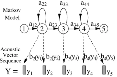
Each base phoneq is represented by a continuous density HMM of

the form illustrated in Figure 2.2 with transition probability param-eters {aij} and output observation distributions {bj()}. In operation,

an HMM makes a transition from its current state to one of its con-nected states every time step. The probability of making a particular 3_{In HTK to ensure that the same number of frames is maintained after adding delta and} delta–delta parameters, the start and end elements are replicated to fill the regression window.

4_{Recognisers often approximate this by amaxoperation so that alternative pronunciations} can be decoded as though they were alternative word hypotheses.

a a a22 a12 a23 a34 a45 33 44 1 2 3 4 5

Y

=

Fig. 2.2 HMM-based phone model.

transition from states_i to states_j is given by the transition probabil-ity {aij}. On entering a state, a feature vector is generated using the

distribution associated with the state being entered,{bj()}. This form

of process yields the standard conditional independence assumptions for an HMM:

• states are conditionally independent of all other states given the previous state;

• observations are conditionally independent of all other obser-vations given the state that generated it.

For a more detailed discussion of the operation of an HMM see [141]. For now, single multivariate Gaussians will be assumed for the out-put distribution:

bj(y) =N(y;µ(j),Σ(j)), (2.7)

whereµ(j) is the mean of state sj and Σ(j) is its covariance. Since the

dimensionality of the acoustic vectoryis relatively high, the covariances

are often constrained to be diagonal. Later inHMM Structure

Refine-ments, the benefits of using mixtures of Gaussians will be discussed.

Given the composite HMM Q formed by concatenating all of the

constituent base phones q(w1)_{, . . . ,q}(wL) _{then the acoustic likelihood is}

given by

p(Y|Q) = θ

2.2 HMM Acoustic Models (Basic-Single Component) 205

where θ=θ0, . . . , θT+1 is a state sequence through the composite

model and p(θ,Y|Q) =aθ0θ1 T t=1 bθt(yt)aθtθt+1. (2.9)

In this equation, θ0 and θT+1 correspond to the non-emitting entry

and exit states shown in Figure 2.2. These are included to simplify the process of concatenating phone models to make words. For simplicity in what follows, these non-emitting states will be ignored and the focus will be on the state sequenceθ1, . . . , θT.

The acoustic model parameters λ= [{aij},{bj()}] can be

effi-ciently estimated from a corpus of training utterances using the forward–backward algorithm [14] which is an example of expectation-maximisation (EM) [33]. For each utteranceY(r), r= 1, . . . , R, of length

T(r)the sequence of baseforms, the HMMs that correspond to the

word-sequence in the utterance, is found and the corresponding composite

HMM constructed. In the first phase of the algorithm, theE-step, the

forward probability α(rj)_t =p(Y_1:t(r), θt=sj;λ) and the backward

prob-ability β_t(ri)=p(Y(r)

t+1:T(r)|θt=si;λ) are calculated via the following

recursions α(rj)_t = i α(ri)_t−1aij bj y(r) t (2.10) β_t(ri) =   j aijbj(y(r)t+1)β (rj) t+1  _, (2.11)

whereiandjare summed over all states. When performing these

recur-sions under-flow can occur for long speech segments, hence in practice the log-probabilities are stored andlog arithmeticis used to avoid this problem [89].5

Given the forward and backward probabilities, the probability of the model occupying statesj at timetfor any given utterancer is just

γ(rj)t =P(θt=sj|Y(r);λ) = 1 P(r)α (rj) t β (rj) t , (2.12)

whereP(r)=p(Y(r);λ). These stateoccupation probabilities, also called

occupation counts, represent a soft alignment of the model states to the data and it is straightforward to show that the new set of Gaussian parameters defined by [83] ˆ µ(j) _{= R} r=1 _T(r) t=1 γ (rj) t y (r) t _R r=1 _T(r) t=1 γ (rj) t (2.13) ˆ Σ(j) = _R r=1 _T(r) t=1 γ (rj) t (y (r) t −µˆ(j))(y (r) t −µˆ(j))T _R r=1 _T(r) t=1 γ (rj) t (2.14)

maximise the likelihood of the data given these alignments. A similar re-estimation equation can be derived for the transition probabilities

ˆ aij = _R r=1P1(r) _T(r) t=1 α (ri) t aijbj(y(r)t+1)β (rj) t+1y (r) t _R r=1 _T(r) t=1 γ (ri) t . (2.15)

This is the second or M-step of the algorithm. Starting from some

initial estimate of the parameters,λ(0), successive iterations of the EM algorithm yield parameter sets λ(1),λ(2), . . . which are guaranteed to improve the likelihood up to some local maximum. A common choice for the initial parameter setλ(0)is to assign the global mean and covariance of the data to the Gaussian output distributions and to set all transition probabilities to be equal. This gives a so-calledflat start model.

This approach to acoustic modelling is often referred to as the

beads-on-a-string model, so-called because all speech utterances are represented by concatenating a sequence of phone models together. The major problem with this is that decomposing each vocabulary word into a sequence of context-independent base phones fails to cap-ture the very large degree of context-dependent variation that exists in real speech. For example, the base form pronunciations for “mood” and “cool” would use the same vowel for “oo,” yet in practice the realisations of “oo” in the two contexts are very different due to the influence of the preceding and following consonant. Context

indepen-dent phone models are referred to asmonophones.

A simple way to mitigate this problem is to use a unique phone model for every possible pair of left and right neighbours. The resulting

2.2 HMM Acoustic Models (Basic-Single Component) 207

models are called triphones and if there areN base phones, there are

N3 potential triphones. To avoid the resulting data sparsity problems,

the complete set of logical triphones L can be mapped to a reduced

set of physical modelsP by clustering and tying together the

param-eters in each cluster. This mapping process is illustrated in Figure 2.3 and the parameter tying is illustrated in Figure 2.4 where the notation

x−q+ydenotes the triphone corresponding to phoneqspoken in the

context of a preceding phone x and a following phone y. Each base

(silence) Stop that (silence)

sil s t oh p th ae t sil m1 m23 m94 m32 m34 m984 m763 m2 m1 W Q L P

sil sil-s+t s- t+oh t-oh+p oh-p+th p-th+ae th-ae+t ae-t+sil sil

Fig. 2.3 Context dependent phone modelling.

t-ih+n t-ih+ng f-ih+l s-ih+l

t-ih+n t-ih+ng f-ih+l s-ih+l Tie similar

states

phone pronunciationq is derived by simple look-up from the pronunci-ation dictionary, these are then mapped to logical phones according to the context, finally the logical phones are mapped to physical models. Notice that the context-dependence spreads across word boundaries and this is essential for capturing many important phonological pro-cesses. For example, the /p/ in “stop that” has its burst suppressed by the following consonant.

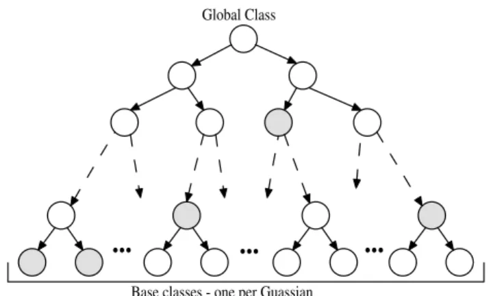
The clustering of logical to physical models typically operates at the state-level rather than the model level since it is simpler and it allows a larger set of physical models to be robustly estimated. The choice of which states to tie is commonly made using decision trees [190]. Each

state position6 of each phone q has a binary tree associated with it.

Each node of the tree carries a question regarding the context. To clus-ter state i of phone q, all states i of all of the logical models derived

from q are collected into a single pool at the root node of the tree.

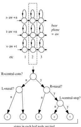
Depending on the answer to the question at each node, the pool of states is successively split until all states have trickled down to leaf nodes. All states in each leaf node are then tied to form a physical model. The questions at each node are selected from a predetermined set to maximise the likelihood of the training data given the final set of state-tyings. If the state output distributions are single component Gaussians and the state occupation counts are known, then the increase in likelihood achieved by splitting the Gaussians at any node can be calculated simply from the counts and model parameters without ref-erence to the training data. Thus, the decision trees can be grown very efficiently using a greedy iterative node splitting algorithm. Figure 2.5 illustrates this tree-based clustering. In the figure, the logical phones s-aw+n and t-aw+n will both be assigned to leaf node 3 and hence they will share the same central state of the representative physical model.7 The partitioning of states using phonetically driven decision trees has several advantages. In particular, logical models which are required but were not seen at all in the training data can be easily synthesised. One disadvantage is that the partitioning can be rather coarse. This 6_{Usually each phone model has three states.}

7_{The total number of tied-states in a large vocabulary speaker independent system typically} ranges between 1000 and 10,000 states.

2.2 HMM Acoustic Models (Basic-Single Component) 209 s- aw +n t-aw +n s- aw +t etc 1 2 3 5 4 3 2 1 n y R=central-cons? y y n n n L=nasal? R=nasal? L=central-stop?

states in each leaf node are tied base phone = aw

Fig. 2.5 Decision tree clustering.

problem can be reduced using so-calledsoft-tying[109]. In this scheme,

a post-processing stage groups each state with its one or two nearest neighbours and pools all of their Gaussians. Thus, the single Gaussian models are converted to mixture Gaussian models whilst holding the total number of Gaussians in the system constant.

To summarise, the core acoustic models of a modern speech recog-niser typically consist of a set of tied three-state HMMs with Gaus-sian output distributions. This core is commonly built in the following steps [189, Ch. 3]:

(1) A flat-start monophone set is created in which each base phone is a monophone single-Gaussian HMM with means and covariances equal to the mean and covariance of the train-ing data.

(2) The parameters of the Gaussian monophones are re-estimated using 3 or 4 iterations of EM.

(3) Each single Gaussian monophone q is cloned once for each

distinct triphonex−q+ythat appears in the training data.

(4) The resulting set of training-data triphones is again

re-estimated using EM and the state occupation counts of the last iteration are saved.

(5) A decision tree is created for each state in each base phone, the training-data triphones are mapped into a smaller set of tied-state triphones and iteratively re-estimated using EM. The final result is the required tied-state context-dependent acoustic model set.

2.3 N-gram Language Models

The prior probability of a word sequence w=w1, . . . , wK required in

(2.2) is given by P(w) = K k=1 P(wk|wk−1, . . . , w1). (2.16)

For large vocabulary recognition, the conditioning word history in

(2.16) is usually truncated to N −1 words to form an N-gram

lan-guage model P(w) = K k=1 P(wk|wk−1, wk−2, . . . , wk−N+1), (2.17)

where N is typically in the range 2–4. Language models are often

assessed in terms of theirperplexity,H, which is defined as

H = − lim K→∞ 1 Klog2(P(w1, . . . , wK)) ≈ − 1 K K k=1 log₂(P(wk|wk−1, wk−2, . . . , wk−N+1)),

where the approximation is used for N-gram language models with a

2.3 N-gram Language Models 211

The N-gram probabilities are estimated from training texts by

counting N-gram occurrences to form maximum likelihood (ML)

parameter estimates. For example, let C(wk−2wk−1wk) represent the

number of occurrences of the three words wk−2wk−1wk and similarly

forC(wk−2wk−1), then

P(wk|wk−1, wk−2)≈C

(wk−2wk−1wk)

C(wk−2wk−1) .

(2.18) The major problem with this simple ML estimation scheme is data sparsity. This can be mitigated by a combination of discounting and

backing-off. For example, using so-calledKatz smoothing [85]

P(wk|wk−1, wk−2) =        dC(w_C(wk−_k−2w_2wk−_k−1w₁₎k) if 0< C≤C C(wk−2wk−1wk) C(wk−2wk−1) if C > C α(wk−1, wk−2)P(wk|wk−1) otherwise, (2.19) where C is a count threshold, C is short-hand for C(wk−2wk−1wk),

d is a discount coefficient and α is a normalisation constant. Thus,

when the N-gram count exceeds some threshold, the ML estimate is

used. When the count is small the same ML estimate is used but dis-counted slightly. The disdis-counted probability mass is then distributed

to the unseenN-grams which are approximated by a weighted version

of the corresponding bigram. This idea can be applied recursively to

estimate any sparse N-gram in terms of a set of back-off weights and

(N−1)-grams. The discounting coefficient is based on the Turing-Good

estimated= (r + 1)nr+1/rnr wherenr is the number ofN-grams that

occur exactly r times in the training data. There are many variations

on this approach [25]. For example, when training data is very sparse, Kneser–Ney smoothing is particularly effective [127].

An alternative approach to robust language model estimation is to

use class-based models in which for every word wk there is a

corre-sponding classck [21, 90]. Then,

P(w) =

K

k=1

P(wk|ck)p(ck|ck−1, . . . , ck−N+1). (2.20)

As for word based models, the classN-gram probabilities are estimated

data sparsity is much less of an issue. The classes themselves are chosen to optimise the likelihood of the training set assuming a bigram class model. It can be shown that when a word is moved from one class to another, the change in perplexity depends only on the counts of a relatively small number of bigrams. Hence, an iterative algorithm can be implemented which repeatedly scans through the vocabulary, testing each word to see if moving it to some other class would increase the likelihood [115].

In practice it is found that for reasonably sized training sets,8 _an

effective language model for large vocabulary applications consists of a smoothed word-based 3 or 4-gram interpolated with a class-based trigram.

2.4 Decoding and Lattice Generation

As noted in the introduction to this section, the most likely word sequence ˆwgiven a sequence of feature vectorsY1:T is found by

search-ing all possible state sequences arissearch-ing from all possible word sequences for the sequence which was most likely to have generated the observed

data Y_1:T. An efficient way to solve this problem is to use dynamic

programming. Letφ(j)t = maxθ{p(Y1:t, θt=sj;λ)}, i.e., the maximum

probability of observing the partial sequence Y_1:t and then being in

statesj at timet given the model parameters λ. This probability can

be efficiently computed using the Viterbi algorithm [177] φ(j)t = max i φ(i)_t−1aij bj(yt). (2.21)

It is initialised by setting φ(j)0 to 1 for the initial, non-emitting, entry

state and 0 for all other states. The probability of the most likely word sequence is then given by maxj{φ(j)_T } and if every maximisation

decision is recorded, a traceback will yield the required best matching state/word sequence.

In practice, a direct implementation of the Viterbi algorithm becomes unmanageably complex for continuous speech where the topol-ogy of the models, the language model constraints and the need to 8_i.e.107 _words.

2.4 Decoding and Lattice Generation 213

bound the computation must all be taken into account. N-gram

lan-guage models and cross-word triphone contexts are particularly prob-lematic since they greatly expand the search space. To deal with this, a number of different architectural approaches have evolved. For Viterbi decoding, the search space can either be constrained by maintaining multiple hypotheses in parallel [173, 191, 192] or it can be expanded dynamically as the search progresses [7, 69, 130, 132]. Alternatively, a completely different approach can be taken where the breadth-first approach of the Viterbi algorithm is replaced by a depth-first search. This gives rise to a class of recognisers calledstack decoders. These can be very efficient, however, because they must compare hypotheses of different lengths, their run-time search characteristics can be difficult to control [76, 135]. Finally, recent advances in weighted finite-state transducer technology enable all of the required information (acoustic models, pronunciation, language model probabilities, etc.) to be inte-grated into a single very large but highly optimised network [122]. This approach offers both flexibility and efficiency and is therefore extremely useful for both research and practical applications.

Although decoders are designed primarily to find the solution to (2.21), in practice, it is relatively simple to generate not just the most

likely hypothesis but theN-best set of hypotheses.N is usually in the

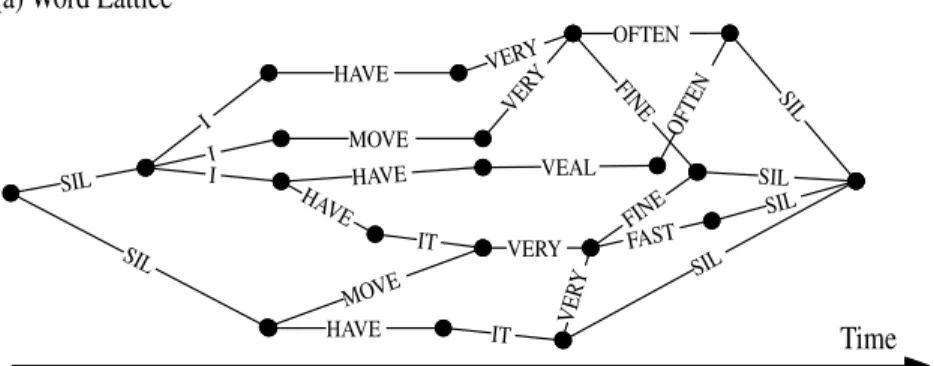
range 100–1000. This is extremely useful since it allows multiple passes over the data without the computational expense of repeatedly solving (2.21) from scratch. A compact and efficient structure for storing these hypotheses is theword lattice [144, 167, 187].

A word lattice consists of a set of nodes representing points in time and a set of spanning arcs representing word hypotheses. An example is shown in Figure 2.6 part (a). In addition to the word IDs shown in the figure, each arc can also carry score information such as the acoustic and language model scores.

Lattices are extremely flexible. For example, they can be rescored by using them as an input recognition network and they can be expanded to allow rescoring by a higher order language model. They can also be

compacted into a very efficient representation called a confusion

net-work [42, 114]. This is illustrated in Figure 2.6 part (b) where the “-”

HAVE HAVE HA VE I I MOVE VERY VER Y I SIL SIL VEAL OFTEN OFTEN SIL SIL SIL SIL FINE IT _VERY FAST VER Y MOVE HAVE _IT

(a) Word Lattice

I HAVE IT VEAL FINE

- MOVE - VERY OFTEN

FAST

(b) Confusion Network

Time

FINE

Fig. 2.6 Example lattice and confusion network.

longer correspond to discrete points in time, instead they simply enforce word sequence constraints. Thus, parallel arcs in the confusion network do not necessarily correspond to the same acoustic segment. However, it is assumed that most of the time the overlap is sufficient to enable parallel arcs to be regarded as competing hypotheses. A confusion net-work has the property that for every path through the original lattice, there exists a corresponding path through the confusion network. Each arc in the confusion network carries the posterior probability of the

corresponding word w. This is computed by finding the link

probabil-ity of w in the lattice using a forward–backward procedure, summing

over all occurrences of w and then normalising so that all competing

word arcs in the confusion network sum to one. Confusion networks can be used for minimum word-error decoding [165] (an example of min-imum Bayes’ risk (MBR) decoding [22]), to provide confidence scores and for merging the outputs of different decoders [41, 43, 63, 72] (see

3

HMM Structure Refinements

In the previous section, basic acoustic HMMs and their use in ASR sys-tems have been explained. Although these simple HMMs may be ade-quate for small vocabulary and similar limited complexity tasks, they do not perform well when used for more complex, and larger vocabulary tasks such as broadcast news transcription and dictation. This section describes some of the extensions that have been used to improve the performance of ASR systems and allow them to be applied to these more interesting and challenging domains.

The use of dynamic Bayesian networks to describe possible exten-sions is first introduced. Some of these extenexten-sions are then discussed in detail. In particular, the use of Gaussian mixture models, effi-cient covariance models and feature projection schemes are presented. Finally, the use of HMMs for generating, rather than recognising, speech is briefly discussed.

3.1 Dynamic Bayesian Networks

InArchitecture of an HMM-Based Recogniser, the HMM was described as a generative model which for a typical phone has three emitting

a₂₂ a₃₃ a₄₄

2 3 4 5

1 a12 a23 a34 a45

y

y

θ

θ

Fig. 3.1 Typical phone HMM topology (left) and dynamic Bayesian network (right).

states, as shown again in Figure 3.1. Also shown in Figure 3.1 is an

alternative, complementary, graphical representation called adynamic

Bayesian network (DBN) which emphasises the conditional dependen-cies of the model [17, 200] and which is particularly useful for describ-ing a variety of extensions to the basic HMM structure. In the DBN notation used here, squares denote discrete variables; circles continu-ous variables; shading indicates an observed variable; and no shading an unobserved variable. The lack of an arc between variables shows conditional independence. Thus Figure 3.1 shows that the observations generated by an HMM are conditionally independent given the unob-served, hidden, state that generated it.

One of the desirable attributes of using DBNs is that it is simple to show extensions in terms of how they modify the conditional indepen-dence assumptions of the model. There are two approaches, which may be combined, to extend the HMM structure in Figure 3.1: adding addi-tional un-observed variables; and adding addiaddi-tional dependency arcs between variables.

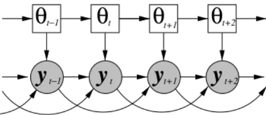
An example of adding additional arcs, in this case between obser-vations is shown in Figure 3.2. Here the observation distribution is

y

y

y

θ

θ

θ

y

θ

Fig. 3.2 Dynamic Bayesian networks for buried Markov models and HMMs with vector linear predictors.

3.2 Gaussian Mixture Models 217

y

y

θ

θ

ω

ω

z

y

y

z

θ

θ

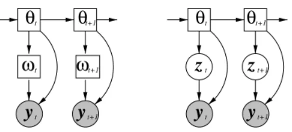
Fig. 3.3 Dynamic Bayesian networks for Gaussian mixture models (left) and factor-analysed models (right).

dependent on the previous two observations in addition to the state that generated it. This DBN describes HMMs with explicit temporal correlation modelling [181], vector predictors [184], and buried Markov models [16]. Although an interesting direction for refining an HMM, this approach has not yet been adopted in mainstream state-of-the-art systems.

Instead of adding arcs, additional unobserved, latent or hidden, vari-ables may be added. To compute probabilities, these hidden varivari-ables must then be marginalised out in the same fashion as the unobserved state sequence for HMMs. For continuous variables this requires a con-tinuous integral over all values of the hidden variable and for discrete variables a summation over all values. Two possible forms of latent vari-able are shown in Figure 3.3. In both cases the temporal dependencies of the model, where the discrete states are conditionally independent of all other states given the previous state, are unaltered allowing the use of standard Viterbi decoding routines. In the first case, the obser-vations are dependent on a discrete latent variable. This is the DBN for an HMM with Gaussian mixture model (GMM) state-output distribu-tions. In the second case, the observations are dependent on a continu-ous latent variable. This is the DBN for an HMM with factor-analysed covariance matrices. Both of these are described in more detail below.

3.2 Gaussian Mixture Models

One of the most commonly used extensions to standard HMMs is to

model the state-output distribution as a mixture model. InArchitecture

to model the state–output distribution. This model therefore assumed that the observed feature vectors are symmetric and unimodal. In prac-tice this is seldom the case. For example, speaker, accent and gender differences tend to create multiple modes in the data. To address this problem, the single Gaussian state-output distribution may be replaced by a mixture of Gaussians which is a highly flexible distribution able to model, for example, asymmetric and multi-modal distributed data.

As described in the previous section, mixture models may be viewed as adding an additional discrete latent variable to the system. The

like-lihood for states_j is now obtained by summing over all the component

likelihoods weighted by their prior

bj(y) = M

m=1

cjmN(y;µ(jm),Σ(jm)), (3.1)

wherecjm is the prior probability for component m of state sj. These

priors satisfy the standard constraints for a valid probability mass func-tion (PMF)

M

m=1

cjm= 1, cjm≥0. (3.2)

This is an example of the general technique of mixture modelling. Each

of the M components of the mixture model is a Gaussian probability

density function (PDF).

Since an additional latent variable has been added to the acoustic model, the form of the EM algorithm previously described needs to be modified [83]. Rather than considering the complete data-set in terms of state-observation pairings, state/component-observations are used. The estimation of the model parameters then follows the same form as

for the single component case. For the mean of Gaussian componentm

of statesj,sjm, ˆ µ(jm)_{= R} r=1 _T(r) t=1 γ (rjm) t y (r) t _R r=1 _T(r) t=1 γ (rjm) t , (3.3)

where γt(rjm)=P(θt=sjm|Y(r);λ) is the probability that component

3.3 Feature Projections 219

R is the number of training sequences. The component priors are

esti-mated in a similar fashion to the transition probabilities.

When using GMMs to model the state-output distribution, variance

flooring is often applied.1 This prevents the variances of the system

becoming too small, for example when a component models a very small number of tightly packed observations. This improves generalisation.

Using GMMs increases the computational overhead since when using log-arithmetic, a series of log-additions are required to compute the GMM likelihood. To improve efficiency, only components which pro-vide a “reasonable” contribution to the total likelihood are included. To further decrease the computational load the GMM likelihood can be approximated simply by the maximum over all the components (weighted by the priors).

In addition, it is necessary to determine the number of components per state in the system. A number of approaches, including discrimina-tive schemes, have been adopted for this [27, 106]. The simplest is to use the same number of components for all states in the system and use held-out data to determine the optimal numbers. A popular alterna-tive approach is based on the Bayesian information criterion (BIC) [27]. Another approach is to make the number of components assigned to the state a function of the number of observations assigned to that state [56].

3.3 Feature Projections

In Architecture for an HMM-Based Recogniser, dynamic first and

second differential parameters, the so-called delta and delta–delta

parameters, were added to the static feature parameters to overcome the limitations of the conditional independence assumption associated with HMMs. Furthermore, the DCT was assumed to approximately decorrelate the feature vector to improve the diagonal covariance approximation and reduce the dimensionality of the feature vector.

It is also possible to use data-driven approaches to decorrelate and reduce the dimensionality of the features. The standard approach is to

use linear transformations, that is

yt=A[p]y˜t, (3.4)

whereA_[p]is ap×dlinear-transform,dis the dimension of the source feature vector ˜y_t, andpis the size of the transformed feature vectory_t. The detailed form of a feature vector transformation such as this

depends on a number of choices. Firstly, the construction of ˜y_t must

be decided and, when required, the class labels that are to be used, for example phone, state or Gaussian component labels. Secondly, the

dimensionalitypof the projected data must be determined. Lastly, the

criterion used to estimateA_[p] must be specified.

An important issue when estimating a projection is whether the class labels of the observations are to be used, or not, i.e., whether the

projection should be estimated in a supervised or unsupervised

fash-ion. In general supervised approaches yield better projections since it is then possible to estimate a transform to improve the discrimination between classes. In contrast, in unsupervised approaches only general attributes of the observations, such as the variances, may be used. How-ever, supervised schemes are usually computationally more expensive than unsupervised schemes. Statistics, such as the means and covari-ance matrices are needed for each of the class labels, whereas unsuper-vised schemes effectively only ever have one class.

The features to be projected are normally based on the standard MFCC, or PLP, feature-vectors. However, the treatment of the delta and delta–delta parameters can vary. One approach is to splice neigh-bouring static vectors together to form a composite vector of typically 9 frames [10] ˜ yt= ysT t−4 ··· ystT ··· yst+4T T . (3.5)

Another approach is to expand the static, delta and delta–delta parameters with third-order dynamic parameters (the difference of delta–deltas) [116]. Both have been used for large vocabulary speech recognition systems. The dimensionality of the projected feature vector is often determined empirically since there is only a single parameter to tune. In [68] a comparison of a number of possible class definitions, phone, state or component, were compared for supervised projection

3.3 Feature Projections 221 schemes. The choice of class is important as the transform tries to ensure that each of these classes is as separable as possible from all others. The study showed that performance using state and compo-nent level classes was similar, and both were better than higher level labels such as phones or words. In practice, the vast majority of systems use component level classes since, as discussed later, this improves the assumption of diagonal covariance matrices.

The simplest form of criterion for estimating the transform is prin-cipal component analysis (PCA). This is an unsupervised projection scheme, so no use is made of class labels. The estimation of the PCA

transform can be found by finding theprows of the orthonormal matrix

Athat maximises Fpca(λ) = log |A_[p]Σ˜gAT_[p]| , (3.6)

where ˜Σg is the total, or global, covariance matrix of the original data,

˜

yt. This selects the orthogonal projections of the data that maximises

the total variance in the projected subspace. Simply selecting subspaces that yield large variances does not necessarily yield subspaces that discriminate between the classes. To address this problem, supervised approaches such as the linear discriminant analysis (LDA) criterion [46] can be used. In LDA the objective is to increase the ratio of the between class variance to the average within class variance for each dimension. This criterion may be expressed as

Flda(λ) = log |A_[p]Σ˜bAT_[p]| |A_[p]Σ˜wAT_[p]| , (3.7)

where ˜Σb is the between-class covariance matrix and ˜Σw the average

within-class covariance matrix where each distinct Gaussian compo-nent is usually assumed to be a separate class. This criterion yields an orthonormal transform such that the average within-class covariance matrix is diagonalised, which should improve the diagonal covariance matrix assumption.

The LDA criterion may be further refined by using the actual class covariance matrices rather than using the averages. One such form is heteroscedastic discriminant analysis (HDA) [149] where the following

criterion is maximised Fhda(λ) = m γ(m)log   |A[p]Σ˜bAT_[p]| |A_[p]Σ˜(m)AT [p]|  _, (3.8)

where γ(m) _{is the total posterior occupation probability for}

compo-nent m and ˜Σ(m) is its covariance matrix in the original space given

by ˜y_t. In this transformation, the matrix A is not constrained to be

orthonormal, and nor does this criterion help with decorrelating the data associated with each Gaussian component. It is thus often used in conjunction with a global semi-tied transform [51] (also known as a maximum likelihood linear transform (MLLT) [65]) described in the next section. An alternative extension to LDA is heteroscedastic LDA (HLDA) [92]. This modifies the LDA criterion in (3.7) in a similar fashion to HDA, but now a transform for the complete feature-space is estimated, rather than for just the dimensions to be retained. The parameters of the HLDA transform can be found in an ML fashion,

as if they were model parameters as discussed in Architecture for an

HMM-Based Recogniser. An important extension of this transform is to ensure that the distributions for all dimensions to be removed are constrained to be the same. This is achieved by tying the parame-ters associated with these dimensions to ensure that they are identical. These dimensions will thus yield no discriminatory information and so need not be retained for recognition. The HLDA criterion can then be expressed as Fhlda(λ) = m γ(m)log   |A|2 diag |A_[d−p]Σ˜gAT_[d−p]| diag |A_[p]Σ˜(m)AT [p]  _, (3.9) where A= A_[p] A_[d−p] . (3.10)

There are two important differences between HLDA and HDA. Firstly, HLDA yields the best projection whilst simultaneously generating the best transform for improving the diagonal covariance matrix approxi-mation. In contrast, for HDA a separate decorrelating transform must

3.4 Covariance Modelling 223 be added. Furthermore, HLDA yields a model for the complete feature-space, whereas HDA only models the useful (non-projected) dimen-sions. This means that multiple subspace projections can be used with HLDA, but not with HDA [53].

Though schemes like HLDA out-perform approaches like LDA they are more computationally expensive and require more memory. Full-covariance matrix statistics for each component are required to estimate an HLDA transform, whereas only the average within and between class covariance matrices are required for LDA. This makes HLDA pro-jections from large dimensional features spaces with large numbers of components impractical. One compromise that is sometimes used is to follow an LDA projection by a decorrelating global semi-tied trans-form [163] described in the next section.

3.4 Covariance Modelling

One of the motivations for using the DCT transform, and some of the projection schemes discussed in the previous section, is to decorrelate the feature vector so that the diagonal covariance matrix approxima-tion becomes reasonable. This is important as in general the use of full covariance Gaussians in large vocabulary systems would be impractical due to the sheer size of the model set.2 Even with small systems, train-ing data limitations often preclude the use of full covariances. Further-more, the computational cost of using full covariance matrices isO(d2)

compared toO(d) for the diagonal case where d is the dimensionality

of the feature vector. To address both of these problems, structured covariance and precision (inverse covariance) matrix representations have been developed. These allow covariance modelling to be improved with very little overhead in terms of memory and computational load.

3.4.1 Structured Covariance Matrices

A standard form of structured covariance matrix arises from factor analysis and the DBN for this was shown in Figure 3.3. Here the

covariance matrix for each Gaussian component m is represented by

(the dependency on the state has been dropped for clarity)

Σ(m)=A(m)_[p] TA(m)_[p] +Σ(m)_diag, (3.11) whereA(m)_[p] is the component-specific, p×d,loading matrixandΣ(m)_diag

is a component specific diagonal covariance matrix. The above expres-sion is based on factor analysis which allows each of the Gaussian com-ponents to be estimated separately using EM [151]. Factor-analysed HMMs [146] generalise this to support both tying over multiple com-ponents of the loading matrices and using GMMs to model the latent variable-space ofz in Figure 3.3.

Although structured covariance matrices of this form reduce the number of parameters needed to represent each covariance matrix, the computation of likelihoods depends on the inverse covariance matrix, i.e., the precision matrix and this will still be a full matrix. Thus, factor-analysed HMMs still incur the decoding cost associated with full covariances.3

3.4.2 Structured Precision Matrices

A more computationally efficient approach to covariance structuring is to model the inverse covariance matrix and a general form for this is [131, 158] Σ(m)−1= B i=1 ν_i(m)S_i, (3.12)

whereν(m) _{is a Gaussian component specific weight vector that}

spec-ifies the contribution from each of the B global positive semi-definite

matrices, Si. One of the desirable properties of this form of model is

that it is computationally efficient during decoding, since log N(y;µ(m),Σ(m)) =−1 2log((2π) d_|Σ(m)_|)− 1 2 B i=1 ν_i(m)(y−µ(m))TSi(y−µ(m)) 3_{Depending on p, the matrix inversion lemmas, also known as the}

3.4 Covariance Modelling 225 =−1 2log((2π) d_|Σ(m)_|) −1 2 B i=1 ν_i(m) yT_S iy−2µ(m)TSiy+µ(m)TSiµ(m) . (3.13)

Thus rather than having the computational cost of a full covariance matrix, it is possible to cache terms such asSiy and yTSiy which do

not depend on the Gaussian component.

One of the simplest and most effective structured covariance rep-resentations is the semi-tied covariance matrix (STC) [51]. This is a specific form of precision matrix model, where the number of bases is

equal to the number of dimensions (B =d) and the bases are

symmet-ric and have rank 1 (thus can be expressed asSi=aT_[i]a[i],a[i]is theith

rowof A). In this case the component likelihoods can be computed by

Ny;µ(m),Σ(m) =|A|N Ay;Aµ(m),Σ(m)_diag (3.14) whereΣ(m)_diag−1 is a diagonal matrix formed from ν(m) and

Σ(m)−1=

d

i=1

ν_i(m)aT_[i]a_[i]=AΣ(m)_diag−1AT. (3.15)

The matrixAis sometimes referred to as the semi-tied transform. One

of the reasons that STC systems are simple to use is that the weight for each dimension is simply the inverse variance for that dimension. The training procedure for STC systems is (after accumulating the standard EM full-covariance matrix statistics):

(1) initialise the transform A(0)=I; setΣ(m0)_diag equal to the

cur-rent model covariance matrices; and set k= 0;

(2) estimate A(k+1) given Σ(mk)_diag ;

(3) set Σ(m(k+1))_diag to the component variance for each dimension using A(k+1);

(4) goto (2) unless converged or maximum number of iterations reached.

During recognition, decoding is very efficient since Aµ(m) is stored

each time instance. There is thus almost no increase in decoding time compared to standard diagonal covariance matrix systems.

STC systems can be made more powerful by using multiple semi-tied transforms [51]. In addition to STC, other types of struc-tured covariance modelling include sub-space constrained precision and means (SPAM) [8], mixtures of inverse covariances [175], and extended maximum likelihood linear transforms (EMLLT) [131].

3.5 HMM Duration Modelling

The probability dj(t) of remaining in state sj fort consecutive

obser-vations in a standard HMM is given by

dj(t) =a_jjt−1(1−ajj), (3.16)

whereajj is the self-transition probability of state sj. Thus, the

stan-dard HMM models the probability of state occupancy as decreasing exponentially with time and clearly this is a poor model of duration.

Given this weakness of the standard HMM, an obvious refinement is to introduce an explicit duration model such that the self-transition loops in Figure 2.2 are replaced by an explicit probability distribution dj(t). Suitable choices for dj(t) are the Poisson distribution [147] and

the Gamma distribution [98].

Whilst the use of these explicit distributions can undoubtably model state segment durations more accurately, they add a very considerable overhead to the computational complexity. This is because the resulting models no longer have the Markov property and this prevents efficient search over possible state alignments. For example, in these so-called

hidden semi-Markov models (HSMMs), the forward probability given in (2.10) becomes α(rj)t = τ i,i=j α(ri)t−τaijdj(τ) τ l=1 bj y(r) t−τ+l . (3.17)

The need to sum over all possible state durations has increased the

complexity by a factor ofO(D2) whereDis the maximum allowed state

duration, and the backward probability and Viterbi decoding suffer the same increase in complexity.

3.6 HMMs for Speech Generation 227 In practice, explicit duration modelling of this form offers some small improvements to performance in small vocabulary applications, and minimal improvements in large vocabulary applications. A typical experience in the latter is that as the accuracy of the phone-output distributions is increased, the improvements gained from duration modelling become negligible. For this reason and its computational complexity, durational modelling is rarely used in current systems.

3.6 HMMs for Speech Generation

HMMs are generative models and although HMM-based acoustic mod-els were developed primarily for speech recognition, it is relevant to consider how well they can actually generate speech. This is not only of direct interest for synthesis applications where the flexibility and compact representation of HMMs offer considerable benefits [168], but it can also provide further insight into their use in recognition [169].

The key issue of interest here is the extent to which the dynamic delta and delta–delta terms can be used to enforce accurate trajectories for the static parameters. If an HMM is used to directly model the speech features, then given the conditional independence assumptions

from Figure 3.1 and a particular state sequence,θ, the trajectory will

be piece-wise stationary where the time segment corresponding to each state, simply adopts the mean-value of that state. This would clearly be a poor fit to real speech where the spectral parameters vary much more smoothly.

TheHMM-trajectory model4 aims to generate realistic feature

tra-jectories by finding the sequence of d-dimensional static observations

which maximises the likelihood of the complete feature vector (i.e. stat-ics + deltas) with respect to the parameters of a standard HMM model. The trajectory of these static parameters will no longer be piecewise stationary since the associated delta parameters also contribute to the likelihood and must therefore be consistent with the HMM parameters. To see how these trajectories can be computed, consider the case of using a feature vector comprising static parameters and “simple

difference” delta parameters. The observation at timetis a function of the static features at timest−1,t and t+ 1

yt= ys t ∆ys_t = 0 I 0 −I 0 I  y s t−1 ys t ys t+1  _, (3.18)

where 0 is a d×d zero matrix and I is a d×didentity matrix. ys_t is the static element of the feature vector at timetand ∆ys_tare the delta features.5

Now if a complete sequence of features is considered, the following

relationship can be obtained between the 2T d features used for the

standard HMM and theT d static features

Y1:T =AYs. (3.19)

To illustrate the form of the 2T d×T d matrix A consider the

obser-vation vectors at times, t−1, t and t+ 1 in the complete sequence.

These may be expressed as

        .. . yt−1 y_t yt+1 .. .         =          ··· 0 I 0 0 0 ··· ··· −I 0 I 0 0 ··· ··· 0 0 I 0 0 ··· ··· 0 −I 0 I 0 ··· ··· 0 0 0 I 0 ··· ··· 0 0 −I 0 I ···                       .. . ys t−2 ys t−1 ys t ys t+1 ys t+2 .. .              . (3.20)

The features modelled by the standard HMM are thus a linear trans-form of the static features. It should therefore be possible to derive the probability distribution of the static feature distribution if the param-eters of the standard HMM are known.

The process of finding the distribution of the static features is

sim-plified by hypothesising an appropriate state/component-sequenceθfor

the observations to be generated. In practical synthesis systems state duration models are often estimated as in the previous section. In this 5_{Here a non-standard version of delta parameters is considered to simplify notation. In this}

3.6 HMMs for Speech Generation 229 case the simplest approach is to set the duration of each state equal to its average (note only single component state-output distributions can

be used). Given θ, the distribution of the associated static sequences

Ys _{will be Gaussian distributed. The likelihood of a static sequence}

can then be expressed in terms of the standard HMM features as 1 Zp(AY s_{|θ;λ) =} 1 ZN(Y1:T;µθ,Σθ) =N(Y s_;µs θ,Σsθ), (3.21)

where Z is a normalisation term. The following relationships exist

between the standard model parameters and the static parameters

Σs_θ−1 = ATΣ−_θ1A (3.22) Σs_θ−1µs_θ = ATΣ−_θ1µ_θ (3.23) µsT θ Σsθ−1µ s θ = µTθΣ−θ1µθ, (3.24)

where the segment mean, µ_θ, and variances,Σ_θ, (along with the

cor-responding versions for the static parameters only,µs_θ and Σs_θ) are

µθ=    µ(θ1) .. . µ(θT)   , Σ_θ=    Σ(θ1) _{··· 0} .. . . .. ... 0 ··· Σ(θT)   . (3.25)

Though the covariance matrix of the HMM features,Σ_θ, has the

block-diagonal structure expected from the HMM, the covariance matrix of the static features,Σs_θ in (3.22), does not have a block diagonal

struc-ture sinceAis not block diagonal. Thus, using the delta parameters to

obtain the distribution of the static parameters does not imply the same conditional independence assumptions as the standard HMM assumes in modelling the static features.

The maximum likelihood static feature trajectory, ˆYs, can now be

found using (3.21). This will simply be the static parameter segment

mean,µs

θ, as the distribution is Gaussian. To find µsθ the relationships

in (3.22) to (3.24) can be rearranged to give ˆ Ys=µs_θ = ATΣ−_θ1A ₋1 ATΣ−_θ1µ_θ. (3.26)

These are all known as µ_θ and Σθ are based on the standard HMM

structured-nature ofAefficient implementations of the matrix inversion may be found.

The basic HMM synthesis model described has been refined in a couple of ways. If the overall length of the utterance to synthesise is

known, then an ML estimate of θ can be found in a manner similar

to Viterbi. Rather than simply using the average state durations for the synthesis process, it is also possible to search for the most likely state/component-sequence. Here ˆ Ys,θˆ = arg max Ys ,θ 1 Zp(AY s_|θ;λ) P(θ;λ) ! . (3.27)

In addition, though the standard HMM model parameters, λ, can be

trained in the usual fashion for example using ML, improved perfor-mance can be obtained by training them so that when used to generate sequences of static features they are a “good” model of the training data. ML-based estimates for this can be derived [168]. Just as regu-lar HMMs can be trained discriminatively as described later, HMM-synthesis models can also be trained discriminatively [186]. One of the major issues with both these improvements is that the Viterbi algo-rithm cannot be directly used with the model to obtain the state-sequence. A frame-delayed version of the Viterbi algorithm can be used [196] to find the state-sequence. However, this is still more expen-sive than the standard Viterbi algorithm.

HMM trajectory models can also be used for speech recogni-tion [169]. This again makes use of the equalities in (3.21). The

recog-nition output for feature vector sequenceY1:T is now based on

ˆ w= arg max w arg maxθ 1 ZN(Y1:T;µθ,Σθ)P(θ|w;λ)P(w) !! . (3.28) As with synthesis, one of the major issues with this form of

decod-ing is that the Viterbi algorithm cannot be used. In practice N-best

list rescoring is often implemented instead. Though an interesting research direction, this form of speech recognition system is not in widespread use.