PROJECT MANAGEMENT WITH SIMULATION
A critical view on the critical path
Jaap A. Ottjes and Hans P.M. Veeke,
Sub Faculty of Mechanical Engineering and Marine Technology, Fac. OCP
Delft University of Technology
Mekelweg 2, 2628 CD Delft, the Netherlands
e-mail:
[email protected]
,
[email protected]
Key words: project planning; decision support; discrete event simulation
ABSTRACT
A process-oriented simulation approach to project management is proposed which gives realistic statistical information about total project data and about
individual activities as a function of contractual completion-time. The proposed method provides the possibility to define a generic activity network, which is simulated. The activities in the network may have any statistical or tabulated completion-time distribution. A project simulation run consists of a large number of sub-runs each simulating a project realisation. A run provides statistical information with respect to project completion-times, individual activities such as the probability of activities being critical and excess probability of contract time, and information for monitoring contract critical activities during project realisation. A case of aircraft maintenance is elaborated in which the model is used to reduce the number of contract time excesses using a simple rule assigning extra capacity to activities. The rule is based on preliminary analyses and information that is obtained during the project progress.
INTRODUCTION
For many years it has been common practice to support project management by planning techniques such as CPM and Pert (Winston,1991) . During recent decades there has been an increase in the use of simulation to support management decisions, including those in the
field of project management (Veeke 1982), (Lightfoot 2000), (Deschaine 2000). One of the main advantages of using simulation is that in addition to providing realistic statistics of the whole project, all the data of every single project-realisation is available and can be used for further analysis. In practice simulation results may be used to determine the contractual completion date of the project during a quotation-process. For each manager it is clear that this ‘contractual’ duration will not be the shortest time possible, because then the chance of exceeding it would be 100%. In consequence management will decide to offer a project-duration with a specified confidence level of for example 90%. To that end, a realistic project completion-time distribution is needed. After the decision on this project-duration there is a 90% chance of project-duration without any critical path, simply because the finishing time will be shorter than the contractual project-duration.
Management of the project will concentrate on those activities that may still cause a late finish. These “contract critical” activities are not necessarily restricted to the critical path activities of the CPM analysis, but may be activities that were not initially critical at all or only slighty critical. The simulation detects these potentially critical activities providing the means to monitor the right activities during real project-execution.
Next process oriented modelling will be explained (Zeigler, 1985) and the kernel of the network model will be shown in pseudo-code. The actual model is coded in the process-oriented simulation tool TOMAS (Veeke and Ottjes, 2000a and b). The model will be further elaborated and applied to a case of aircraft
maintenance. The results of the modelling will be discussed from a project manager’s point of view.
PROCESS-ORIENTED MODEL
The process-oriented approach used in this work can be summarised in two steps: (Healy, 1997), (Veeke and Ottjes, 1999).
Step 1: decompose the system into relevant classes of elements, preferably patterned on the real-world elements of the system. A class is characterised by its attributes. An instance of a class will be called an
element. The state of each element is defined by the value of its attributes.
Step 2: distinguish the “living” element classes and provide their process description.
A process governs the dynamic behaviour of each element. The system time during a simulation is called
now. In the process description of an element class we use hold t to indicate that an element needs t time units to carry out some task. If such a hold statement is encountered in the process description, the process halts until time t has elapsed and then continues its process. In other words the process is waiting for a specific time event. Analogous to this, it is possible for a process to wait for a state event e.g. for a specific condition to be fulfilled. In pseudo-code this is written as: standby
while/until condition. Another time consuming statement in a process description is suspend meaning that an element becomes passive when this statement is encountered. A passive element can only be restarted by the resume command given from the process of another element. Because several elements may be active at the same time a sequencing mechanism is needed to synchronise the activities and to manage the event calendar. This mechanism must be supported by the simulation package that is used.
Additional features are queues or sets, which may contain elements and, in the case of stochastic behaviour, distributions, modelling for example execution duration. Queues and sets and distributions may be used as attributes of element classes. The kernel of the network model and its dynamics will now be described in terms of a process-oriented model in pseudo-code and in Tomas-code.
THE NETWORK MODEL
We distinguish two element classes: the activity class and the monitor class.
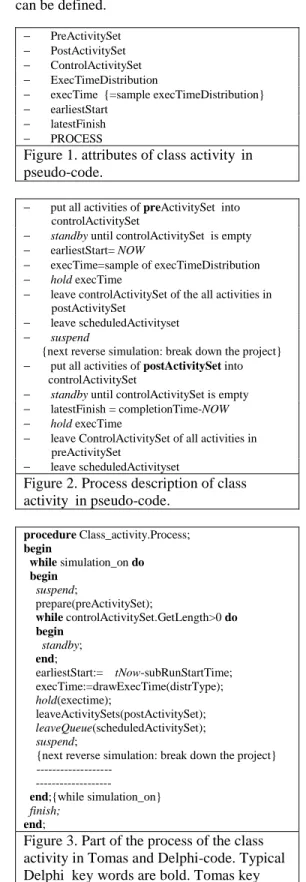
The main element class is the activity class. We use the “activity on node” description. The activity class owns several attributes such as a preActivitySet and
postActivitySet as shown in Figure 1. These sets contain the preceding and succeeding activities respectively. In this way any directed activity network can be defined.
− PreActivitySet
− PostActivitySet
− ControlActivitySet
− ExecTimeDistribution
− execTime {=sample execTimeDistribution}
− earliestStart
− latestFinish
− PROCESS
Figure 1. attributes of class activity in pseudo-code.
− put all activities of preActivitySet into controlActivitySet
− standby until controlActivitySet is empty
− earliestStart= NOW
− execTime=sample of execTimeDistribution
− hold execTime
− leave controlActivitySet of the all activities in postActivitySet
− leave scheduledActivityset
− suspend
{next reverse simulation: break down the project}
− put all activities of postActivitySet into controlActivitySet
− standby until controlActivitySet is empty
− latestFinish = completionTime-NOW
− hold execTime
− leave ControlActivitySet of all activities in preActivitySet
− leave scheduledActivityset
Figure 2. Process description of class activity in pseudo-code. procedure Class_activity.Process; begin while simulation_on do begin suspend; prepare(preActivitySet); while controlActivitySet.GetLength>0 do begin standby; end;
earliestStart:= tNow-subRunStartTime; execTime:=drawExecTime(distrType); hold(exectime);
leaveActivitySets(postActivitySet); leaveQueue(scheduledActivitySet); suspend;
{next reverse simulation: break down the project}
end;{while simulation_on} finish;
end;
Figure 3. Part of the process of the class activity in Tomas and Delphi-code. Typical Delphi key words are bold. Tomas key words are italic.
The controlActivitySet is used for run control purposes. In addition to this an activity owns its execution time distribution, which can be of any type for each instance, and typical data such as earliest start time and latest completion-time, which have to be determined during simulation. An activity owns a PROCESS that takes care of its own timely execution. In other words: the activity waits until it is allowed to be executed. It then executes itself using a sample from its execution time distribution as activity-duration. After execution it leaves the scheduledActivitySet. If all the activities of the project are finished (scheduledActivitySet= empty), the make span and all early start times are known. Then the simulation is performed in reverse. In other words the project is broken down. This provides the latest finish data for all activities. The activity slack (also called total float) is defined as:
slack=latest finish – executionTime - earliest start.
An activity with slack=0 is called critical.
The process of the activity class is described in Figure 2. Figure 3 shows part of the code of the model implementation in Tomas.
For number of sub-runs Do:
− Put all activities into the scheduledActivitySet
− Start processes of all activities
− Standby until scheduledActivitySet is empty
− CompletionTime=NOW
{prepare and start the reverse simulation }
− Put all activities back into the scheduledActivitySet
− Resume processes of all activities
− Standby until scheduledActivitySet is empty
Figure 4. Process description of the class monitor in pseudo-code. 1 1 1 prepare for inspection 1 3 4 5 clean and dismount 3 9 10 12 inspect casco 2 1 1 1 dismount for greasing 4 3 3 3 dismount engines 5 10 28 50 repair casco 6 17 7 7 inspection large wheels 7 6 6 6 inspection nose wheel 8 2 3 4 grease 9 18 18 18 testing instruments 10 1 1 1 clean port engine 11 1 1 1 clean star-board engine 12 6 9 15 repair large wheels 13 6 8 12 repair nose wheel 14 1 1 1 check greasing 15 20 30 50 repair instruments 16 21 24 30 inspect port engine 17 2 2 2 inspect fire extinguish eq. 18 20 23 35 inspect star-board engine 19 1 1 1 test retrack mechanism 20 1 3 7 repair retrack mechanism 24 1 1 1 load emer-gency unit 25 20 36 55 repair port engine 21 8 11 15 repair fire extinguish eq. 22 18 34 60 repair star-board engine 23 0.5 1 1.5 final check 26 lb av ub activity name act.nr
Figure 5. Case: Aircraft maintenance activity network with activitie NRs, name and activity-duration data: lb: lower bound, av: average and ub: upper bound.
lb
av
ub
f2
f1
Figure 6: General execution time distribution for an activity. Three numbers are given: lb: lower bound, av: the average and ub: the upper bound. In order to obtain the average “av” it is demanded that
f1*(av-lb)=f2*(ub-av)
The monitor class governs the simulation runs. Its process is described in Figure 4. The monitor is responsible for the preparation, start and analysing of a simulation run. One simulation run consists of a number of simulation sub-runs. Every sub-run simulates one realisation of the project giving a completion-time and all data of the individual activities. The data of each sub-run is stored for further analysis.
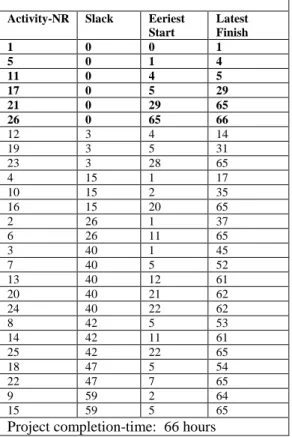
Table 1. Critical path analysis with fixed average activity execution times (av) given in Figure 5. Activity-NR Slack Eeriest
Start Latest Finish 1 0 0 1 5 0 1 4 11 0 4 5 17 0 5 29 21 0 29 65 26 0 65 66 12 3 4 14 19 3 5 31 23 3 28 65 4 15 1 17 10 15 2 35 16 15 20 65 2 26 1 37 6 26 11 65 3 40 1 45 7 40 5 52 13 40 12 61 20 40 21 62 24 40 22 62 8 42 5 53 14 42 11 61 25 42 22 65 18 47 5 54 22 47 7 65 9 59 2 64 15 59 5 65
Project completion-time: 66 hours
One run consequently provides statistical data about project completion-times and the probabilty of activities that are critical. In this work a run consist of 1000-5000 sub-runs. With the approach described
multi-project simulation can be obtained by creating a monitor for each project and starting it at the proper time. In such cases no reverse simulation is performed. Further it is possible to allocate scarce resources (Ottjes and Veeke 2000). This paper focuses on a single project.
APPLYING THE MODEL: A CASE
The use of the model will be illustrated by a simplified case concerning aircraft maintenance (Veeke, 1997). Figure 5 shows the activity network. The activities are named and also identified by a number. The durations of the activities indicated apply to a “general” distribution explained in Figure 6. Any other
distribution function may be applied including functions defined by a table.
Table 2. critical path analysis. The project was simulated 5000 times using activity execution times drawn from the distribution according to the data in Figure 5 and shaped as Figure 6. The last column shows the percentage of sub-runs that the activity was critical in the case of a project completion-time exceeding the contract time. The contract time was set at 84.15 hours being the 90% percentile of the project completion-time distribution. Activity-NR Av.Slack % Critical % Contract Critical 1 0.0 100.000 100.000 26 0.0 100.000 100.000 5 0.5 90.760 100.000 11 5.4 54.300 32.934 17 5.4 54.300 32.934 21 5.4 54.300 32.934 12 8.6 36.460 67.066 19 8.6 36.460 67.066 23 8.6 36.460 67.066 4 20.3 7.600 0.000 10 20.3 7.600 0.000 16 20.3 7.600 0.000 2 31.7 1.640 0.000 6 31.7 1.640 0.000 24 45.2 0.000 0.000 20 45.2 0.000 0.000 3 45.2 0.000 0.000 7 45.6 0.000 0.000 13 45.6 0.000 0.000 25 47.3 0.000 0.000 14 47.6 0.000 0.000 8 47.6 0.000 0.000 18 52.6 0.000 0.000 22 52.6 0.000 0.000 9 64.6 0.000 0.000 15 64.6 0.000 0.000
Average project completion-time: 71.64 hours
Experiments
One run with one sub-run was done using the average activity execution times from Figure 5 as fixed
execution times. Table 1 shows the activities ranked to their slack. The first 6 activities are critical.
Figure 7 shows the completion-time distribution as a result of one run of 5000 sub-runs in which activity execution times are drawn from the individual activity distribution functions. The average completion-time amounts to 71.64 hours, which appears to be
substantially more than the completion-time determined with average execution times. To emphasis the effect of activity-duration distribution, a "worse case" run was performed using exponential distributed activity execution times with the same averages as those given in Figure 5.
Entries 5000 90% Perc entile 84.15 Average 71.64 95% Perc entile 86.40 Stand.D ev. 9.59 Maximum 90.67
0 2 0 0 4 0 0 6 0 0 8 0 0 4 0 4 8 5 6 6 4 7 2 8 0 8 8 9 6
pro jec t c ompletio n time s (h)
frequenc
y
Figure 7. Completion-time distribution as a result of one run of 5000 sub-runs in with activity execution times drawn from the individual activity distribution functions defined by Figure 6 using the parameters of Figure 5. E n tr ie s 5 00 0 9 0% P er c en tile 1 54 .1 2 5 A ve r ag e 9 7 .5 0 9 5 % P e r c e n tile 1 8 0. 59 S ta n d. D e v. 4 3 .4 9 M a xim u m 37 6 .56 0 1 0 0 2 0 0 3 0 0 4 0 0 5 0 0 0 4 8 9 6 1 4 4 1 9 2 2 4 0 2 8 8 3 3 6 3 8 4 pr o je c t c o m p le tio n tim e s ( h) fr equency
Figure 8. Completion-time distribution as a result of one run of 5000 sub-runs in which activity execution times are drawn from the individual activity distribution functions. Here negative exponential distribution functions were applied with average indicated in Figure 5.
The results are shown in Figure 8, and give an average project completion-time of 97.5 hours and a 90% completion-time percentile of 154 hours. It can be
concluded that the completion-time distribution and its average strongly depend on the execution time distributions of the activities. If (some) activity execution time distributions are unknown in practice, experiments with several distribution types provide insight in the influence on completion-time. All further runs in this paper refer to the general distribution type of Figure 6. Table 2 represents the same run as Figure 7 and shows the results for all activities sorted on average slack. In column 3 the percentage of the sub-runs in which the activity was critical is indicated. The project contract time was chosen as the 90% percentile of Figure 8, this being 84.15 hours. The last column shows the percentage in which the activity was critical if the contract time was exceeded. We will call that “contract critical”. Some activities, for example activity 23, are not critical with fixed average execution times but appear to be critical to some extent when using the execution time distributions, and are highly critical if the contact time is exceeded. These activities have to be monitored carefully during the project. From the point of view of a project manager it is very important to know what decisions have to be made during the project. It is necessary to appreciate how to use additional information gained during progress of the project. After activity 19: check starboard engine, there may be a pretty accurate estimate of the duration of activity 23, the repair time of the engine. How to use this extra information! For example, the manager needs to know wether to apply extra resources, speeding up activity 23 in order to avoid project tardiness.
Consequently he needs to know at what execution time level activity 23 will be contract critical. To answer this question runs were performed for a number of pre-set execution times of activity 23. The results are shown in Figure 9. 0 20 40 60 80 100 51 52 53 54 55
execution times of activity 23
%c o n tra c t-c ri ti c a l
Figure 9. Relation between activity 23 being contract critical and its execution time. As a contract time the 90% percentile of the project completion-time distribution was taken this being 84.15 hours. Each measuring point represents a run with 1000 sub-runs.
It can be concluded that if the execution time of activity 23 is kept under 52.7 hours, it will not become critical. The critical activity-duration depends on the used contract time according to Figure 10.
48 50 52 54 56 80 82 84 86 88
project Contract Time
exec. ti m e of act . 23
Figure 10. Critical levels of duration of activity 23 as a function of the project contract time. The contract time values correspond with percentiles of 80%, 85%, 90% and 95% (see also Figure 7).
Capacity
Another aspect for which simulation offers added value is the assignment of finite capacity. Most networks only reflect the technical limitations imposed on the activity-sequence. So two activities that have no technical dependencies may be executed in parallel in the network. Limited capacity may prevent or delay parallel execution. However, it is clear that at each moment the need for capacity is determined by the duration of the preceding activities and the actual need for capacity. Simulation offers a natural way of dealing with limited capacities by dynamically assigning capacity to activities according priority rules.
− if (exectime>ultimateValue) then
− begin
− if mechanic available then
− begin − claim mechanic − exectime:=exectime*2/3 − end − end − hold execTime
− eventually release mechanic
Figure 11. Pseudo-code capacity claiming rule replacing "hold execTime" statement in Figure 2 To illustrate this the case under consideration will be further elaborated. We will focus on the two engine repair activities 21 and 23. The duration of these activities is based on two mechanics working per activity. We assume these two mechanics are available for each engine. As shown in Figure 9, activity 23 may have to be speeded up to remain under an ultimate value
(52.7 hours). To this end the rule is that an additional mechanic is brought in if the repair time, as predicted in the preceding inspection activity, exceeds the ultimate value. It is necessary to determine how many additional mechanics are needed and how the rule influences the completion-times. First the ultimate value of activity 21 is determined in a way similar that used for activity 23. The rule was implemented in the activity process as indicated in Figure 11.
Two types of experiments were performed:
1: infinite capacity; in this case two extra mechanics are available
2: restricted capacity: one extra mechanic is available The results are shown in Table 3 and Figure 12.
Table 3. Experiments with capacity rule. Each run consists of 5000 sub-runs. The contract time applied was 84.15, this being the 90% percentile of the completion-time distribution without the rule given in Figure 7.
infinite extra capacity finite extra capacity No extra capacity % exceeding contract time 0 1 10 %interventions 29 27 0 average project completion-time 67.55 67.88 71.64 std. Deviation 6.86 7.23 9.59 max completion-time 83.92 89.56 90.67
0
400
800
1200
52
64
76
88
100
project completion times (h)
fr
equency
Entries 5000 90% Percentile 77.88 Average 67.88 95% Percentile 80.25 Stand.Dev. 7.23 M aximum 89.56
Figure 12. Completion-time distribution as a result of one run of 5000 sub-runs with one extra mechanic who is assigned to activity 21 or 23 according the rule explained in Figure 11.
The experiments indicated that the risk of contract time excess can be reduced from 10% to 1% with one extra mechanic scheduled according the rule. Of course evaluation of cost should determine wether such a measure is indeed profitable.
CONCLUSIONS
Process-oriented simulation offers a natural way for project planning, especially with respect to uncertainty about the duration of activities and all kinds of specific constraints in and between activities. If activity-duration distributions are known, simulation provides realistic statistics on project duration and information about the chance of individual activities being critical. A case relating aircraft maintenance shows a very large influence of activity-duration distribution functions on average project completion-time and its distribution. If the distribution functions of one ore more activity durations are unknown, experiments with several distribution types supplies insight in completion-time distributions. From the completion-time distribution function a project contract time with known probability can be derived. When this contract time is aggreed, further experiments indicate contract critical activities. Analysing the influence of these activities provides criteria for when and how to intervene during the progress of the project in order to force the completion of the project within the contract time. Further research will focus on the allocation of capacity and resource allocation.
REFERENCES
Deschaine, L.M., Pack, S.R., Zafran, F.A., Patet, J.J. 2000. “Project Risk Quantifier and optimal Project Accelerator- Using Machine Learning and Stochastic Simulation to Optimize Project Completion Dates and Costs”. In Proceedings of Advanced Simulation Technology Conference (ASTC2000). April 16-20, 2000, Washington, D.C. pp.157-162. The Society for Computer Simulation International (SCS), ISBN: 1-56555-199-0
Healy, J. R.A. Kilgore 1997. "Silk,: A Java-Based Process Simulation Language". in Proceedings of the 1997 Winter Simulation Conference, IEEE,
Lightfoot, J. 2000. “Wing Structure Assembly Processes Using Simulation”.In proceedings of Advanced Simulation Technology Conference (ASTC2000). April 16-20, 2000, Washington, D.C. pp.157-162. The Society for Computer Simulation International (SCS), ISBN: 1-56555-199-0 Ottjes, Jaap A. and Hans P.M. Veeke. 2000 .
“Production scheduling of complex jobs with simulation”. In proceedings of Advanced Simulation Technology Conference (ASTC2000) April 16-20,
2000, Washington, D.C. pp.157-162. The Society for Computer Simulation International (SCS), ISBN: 1-56555-199-0.
Veeke, H.P.M. 1982. "Process simulation as a management Tool, Proceedings of the IASTED International Symposium Applied Modelling and Simulation, Paris, 1982.
Veeke, H.P.M. 1997. “Customer based production control”. MB-Produktietechniek( in Dutch), vol:63:8/9
pp.246-264, 1997.
Veeke, H.P.M. and Ottjes, J.A. 1999. “Problem oriented modelling and simulation”, Proc. 1999 Summer computer Simulation Conference (SCS’99) Chicago, Illinois pp.110-114, ISBN 1-56555-173-7 Veeke, Hans P.M., Jaap A. Ottjes, 2000a. TomasWeb: web site: www.tomasweb.com
Veeke, Hans P.M., Jaap A. Ottjes, 2000b. Tomas: Tool for Object-oriented Modelling And Simulation. In
proceedings of Advanced Simulation Technology Conference (ASTC2000). April 16-20, 2000,
Washington, D.C. pp. 76-81. The Society for Computer Simulation International (SCS), ISBN: 1-56555-199-0 Winston, W.L. 1991. Operations Research
Applications and Algorithms, 2ed., PWS-KENT Publishing Company Boston, ISBN:0-534-98079-1 Zeigler, B.P. 1985. Theory of Modeling and Simulation. Krieger, Malaba.