EVOLUTION OF A STORM-DRIVEN CLOUDY BOUNDARY LAYER IN THE ARCTIC
JUN INOUE1;*, BRANKO KOSOVIC´2 and JUDITH A. CURRY1
1School of Earth and Atmospheric Sciences, Georgia Institute of Technology, 311 Ferst Dr., Atlanta, GA 30332-0340, U.S.A.;2Lawrence Livermore National Laboratory Livermore, CA, U.S.A.
(Received in final form 1 April 2004)
Abstract. To investigate the processes of development and maintenance of low-level clouds
during major synoptic events, the cloudy boundary layer under stormy conditions during the summertime Arctic has been studied using observations from the Surface Heat Budget of the Arctic Ocean (SHEBA) experiment and large-eddy simulations (LES). On 29 July 1998, a stable Arctic cloudy boundary-layer event was observed after the passage of a synoptic low pressure system. The local dynamic and thermodynamic structure of the boundary layer was determined from aircraft measurements including the analysis of turbulence, cloud micro-physics and radiative properties. After the upper cloud layer advected over the existing cloud layer, the turbulent kinetic energy (TKE) budget indicated that the cloud layer below 200 m was maintained predominantly by shear production. Observations of longwave radiation showed that cloud-top cooling at the lower cloud top has been suppressed by radiative effects of the upper cloud layer. Our LES results demonstrate the importance of the combination of shear mixing near the surface and radiative cooling at the cloud top in the storm-driven cloudy boundary layer. Once the low-level cloud reaches a certain height, depending on the amount of cloud-top cooling, the two sources of TKE production begin to separate in space under continuous stormy conditions, suggesting one possible mechanism for the cloud layering. The sensitivity tests suggest that the storm-driven cloudy boundary layer is possibly switched to the shear-driven system due to the advection of upper clouds or to the buoyantly driven system due to the lack of wind shear. A comparison is made of this storm-driven boundary layer with the buoyantly driven boundary layer previously described in the literature.
Keywords: Radiative cooling, Shear mixing, SHEBA, Storm-driven boundary layer.
1. Introduction
Persistent stratus cloud layers over the Arctic Ocean are important modu-lators of the climate through their effect on atmospheric radiation and ver-tical turbulent transfer of heat, moisture and momentum in the boundary layer. Understanding the effect of clouds on the surface is an especially vital issue because it can significantly impact upon the melting, refreezing, thick-ness and distribution of sea ice (e.g., Maykut and Untersteiner, 1971). There are many physical processes related to clouds over the Arctic region that are still poorly understood (Bromwich et al., 1994; Curry et al., 1996).
DOI 10.1007/s10546-004-6003-2
Summertime Arctic stratus clouds are believed to be typically formed in relatively warm and moist continental air as it flows over the pack ice. Condensation is induced by radiative and diffusive cooling to the colder surface and longwave emission to space (Herman and Goody, 1976). Such a stable boundary layer is typically characterized by strong wind shear over the ice cover (e.g., Bru¨mmer et al., 1994). In addition, this stable stratification sometimes can be coupled with stratus clouds (e.g., Curry et al., 1988) and can often extend over several days (Curry et al., 1996). Once the surface fog or cloud forms, vertical mixing occurs due to cloud-top radiative cooling. Analyzing a series of 12 vertical profiles in a variety of boundary-layer stratus clouds in the summertime Arctic, Herman and Curry (1984) found that the observed low-level stratus cloud tops were typically 1000 m high and buoy-antly driven. Some common features were also found in North Sea strato-cumulus (Nicholls, 1984). The radiatively driven cloud-topped boundary layer is often found to be decoupled from the surface (Nicholls and Leighton, 1986).
Mid- and upper-level clouds associated with synoptic frontal systems are sometimes advected over existing lower-level clouds in the summertime Arctic. From a statistical study based on radar and lidar data from the Surface Heat Budget of the Arctic Ocean (SHEBA) experiment, Intrieri et al. (2002) found that one of the highest frequency of the occurrence of cloud-top appears between heights of 6 and 8 km. These upper clouds may cause the decay of the lower clouds through suppression of cloud-top radiative cooling. Although cyclonic events drive the seasonal transition through changes in numerous surface energy budget terms, the surface temperature, and the number and spatial coverage of open leads (Ruffieux et al., 1995; Curry et al., 2002; Persson et al., 2002), the combination of turbulent and radiative properties related to the ‘storm-driven boundary layer’ is still poorly understood.
To understand the complicated structure of cloud layering that has been observed frequently in the summertime Arctic, modelling studies focusing on the radiative transfer in the boundary layer have been conducted for the summertime Arctic boundary layer and formation of multiple cloud layers (Herman and Goody, 1976; McInnes and Curry, 1995). Large-eddy simula-tion (LES) is also a useful tool to investigate the impact of turbulence on the boundary layer more explicitly. In LES large eddies, which contain most of the energy and dominate turbulent fluxes within the boundary layer, are explicitly simulated while subgrid-scale motions are parameterized. In recent years, the stably stratified boundary layer has been studied with a LES model (Mason and Derbyshire, 1990; Andren, 1995; Kosovic´ and Curry, 2000; Saiki et al., 2000; Otte and Wyngaard, 2001).
The goal of our study is to propose conceptual models for the evolution of the storm-driven boundary layer in the summertime Arctic. For this purpose,
we use aircraft observations from SHEBA, which was a year-long field program that employed a drifting ship station on the pack ice of the Arctic Ocean, in combination with remote sensing, aircraft observations and modelling analyses of the entire Arctic Basin (Perovich et al., 1999; Curry et al., 2000; Uttal et al., 2002). We focus on the observations of 29 July 1998 when a stable boundary layer with surface cloud was observed, and simulate the boundary-layer structure with a LES model (Kosovic´ and Curry, 2000). Section 2 presents a description of the observations. The turbulent charac-teristics and radiative properties observed are shown in Section 3, the physical processes of the stormy boundary layer are investigated using LES in Section 4, and finally, we present a summary and conclusions in Section 5.
2. Observations
2.1. AIRCRAFT DATA
The National Center for Atmospheric Research (NCAR) C-130 Research Aircraft at the SHEBA ship at 78.50° N, 163.20° W flew on 29 July 1998 after passage of a low pressure system over the Arctic Ocean. The main objective of this flight was to obtain meteorological data within a cloudy boundary layer under stormy conditions. The capabilities of the NCAR C-130 and the instrumentation on the aircraft are described in detail in Curry et al. (2000). The location of the flight is depicted in Figure 1. The flight pattern
Figure 1. AVHRR infrared satellite image on 1900 UTC 29 July 1998. The location of the SHEBA ship is depicted by a closed square.
consisted of six level flights at least 30 km long below the 600 m level between 2213 and 2304 UTC on 29 July, and two vertical soundings before and after these level flights.
Measurements of atmospheric temperature, dew point, humidity, winds, turbulence, radiative fluxes, and microphysical data were obtained from the aircraft. Fast response (25 Hz) temperature, water vapour, and velocity data were collected with a Rosemount thermometer, Lyman-alpha hygrometer, and gust probes, respectively. The processes for the determination of vari-ances and covarivari-ances will be described in Section 3.1. Upward and down-ward shortwave and longwave broadband radiative fluxes were obtained with Eppley pyranometers and pyrgeometers. The King probe measured cloud liquid water content (LWC).
To grasp the synoptic situation, Advanced Very High Resolution Radi-ometer (AVHRR) satellite imagery and National Centers for Environmental Prediction (NCEP) reanalyses were used in this study. Ancillary datasets include cloud radar images obtained at the SHEBA ship, which was specif-ically designed by NOAA Environmental Technology Laboratory (ETL) for long-term continuous operation under Arctic conditions with an emphasis on
(a)
(b)
(c)
(d)
Figure 2. Time series of (a) surface pressure, (b) air temperature at 10-m level, and (c) albedo obtained by the SHEBA tower, and (d) horizontal distribution of air temperature and wind fields at 1000 hPa by NCEP reanalyses for 1800 UTC 29 July 1998. Dotted contour denotes 80%of the ice concentration. The asterisk indicates the location of the SHEBA ship and flight campaign. The grey area denotes temperatures below 274 K. Dashed lines denote the period of 29 July 1998.
the detection of Arctic clouds (Shupe et al., 2001; Intrieri et al., 2002). Meteorological tower data from the Atmospheric Surface Flux Group (ASFG) site and the sounding data from the GPS/Loran Atmospheric Sounding System (GLASS) are also used in our study.
2.2. SYNOPTICSITUATION
In July and August 1998, the SHEBA camp was located on the pack ice in the Chukchi Sea near 78° N, 161–166° W. During these two months, several cyclonic events occurred, producing significant reduction in surface pressure (Figure 2a). In particular, from 26 July to 31 July, surface pressure and air temperature decreased 35 hPa and 2 K, respectively (Figure 2a and b). During this period, the precipitation changed from rain to ice pellets; at 2300 UTC on 28 July, graupel or small hail (25 mm in diameter) were reported from the ship. Finally, precipitation changed to snow near 1200 UTC on 29 July. As the result of the substantial ice divergence caused by strong winds, the lead fraction increased from 5%to 14% (Curry et al., 2002). Al-though Persson et al. (2002) reported that the onset of freezing started on 16 August 1998, passage of the cyclone at the end of July caused an increase in albedo (Figure 2c) through the glazing of surface melt ponds associated with a fall in surface air temperature and the accumulation of some snow on the ice (Curry et al., 2002).
The underlying surface consisted of melting multi-year sea ice. The fraction of open water in the vicinity of the observations was about 6%, and the surface melt pond coverage was about 30%. While the surface was heterogeneous in physical characteristics, the temperature of the sur-face was homogeneous, at the melting point. Although small sursur-face temperature variations in melting sea ice can arise owing to surface solar heating in leads and in melt ponds, such variations did not occur in this situation owing to the heavy cloud cover and relatively strong surface winds.
On 29 July 1998, low-level clouds behind the frontal system are evident in the infrared AVHRR satellite imagery (Figure 1), associated with cold advection behind the frontal system (Figure 2d). Figure 3 shows the time–height cross-section of the cloud radar reflectivity at the SHEBA site and coordinates of the boundary-layer flight pattern over the SHEBA site. The boundary layer decayed when the upper clouds were advected into the region (2015–2300 UTC). However, according to the profiles of potential temperature obtained by radiosondes before the aircraft observations (dotted lines in Figure 4a), the boundary layer deepened from 200 to 700 m between 1200 UTC 28 July and 1200 UTC 29 July.
2.3. MEAN PROFILES
The vertical profiles of potential temperature, wind components, water va-pour mixing ratio and liquid water content (LWC) during vertical descent and ascent of the aircraft are plotted in Figure 4 along with the horizontal leg average profiles. The scatter among the instantaneous profiles is indicative of Figure 3. Time–height cross-sections of radar reflectivity at the SHEBA site and flight coor-dinate of C-130 over the site on 29 July 1998.
0.0 0.5 1.0 1.5 2.0 2.5 Height [km] 270 280 290 θ[κ] 1 2 3 4 (a) 5 10 15 20 U-Wind [m s ] (b) -10 -5 0 5 V-Wind [m s ] (c) 2 3 4 5 Mixing ratio [g kg ] (d) 0.0 0.5 1.0 1.5 2.0 2.5 0.0 0.1 0.2 0.3 LWC [g m ] (e)
Figure 4. Profiles of (a) potential temperature (K), (b) uand (c) vwind (m s1), (d) water
vapour mixing ratio (g kg1) and (e) LWC (g m3) obtained from the aircraft descent and ascent for 2200–2215 UTC (thick line) and 2315–2330 UTC (thin line) on 29 July. The circles represent leg-average values. Sounding data obtained from GLASS are depicted by dotted lines. SHEBA tower data at the 10-m level are depicted by closed triangles for 2300 UTC.
horizontal and temporal variability. The SHEBA tower data at 10 m for 2300 UTC is also provided to support the continuity of the aircraft profiles near the surface (closed triangles in Figure 4).
The boundary layer at 2200 UTC is characterized by two inversion layers associated with upper clouds at 2100 m and lower clouds below 500 m. The wind is westerly, categorized as a cold advection regime behind a frontal system. It is noted that the u wind component has strong shear near the surface below the 200 m level; there is also significant wind shear in the v
wind component between 300 and 500 m. Water vapour increases with height through the lower cloud layer reaching a peak value near 400 m.
After an hour (2300 UTC) the inversion layer at 500 m decreases about 50 m as seen in Figure 4; the maximum water vapour mixing ratio also decreased from 4.7 to 4.2 g kg1. This tendency can be also seen in LWC, in particular, the upper half of the layer decayed significantly from 0.3 to 0.2 g m3. However, the characteristics of wind components persist during
the observation.
3. Turbulent and Radiative Properties of the Cloudy Boundary Layer
In this section, the turbulent and radiative properties of the cloudy boundary layer are examined using profiles of variances, turbulent heat and momentum fluxes, turbulent kinetic energy (TKE), and longwave radiation.
3.1. VARIANCES, FLUXES, AND TKE BUDGET
Spectra and cospectra are calculated from the high-frequency temperature and velocity data collected during each leg of the aircraft flight, following Pinto (1998). The time series of each variable is partitioned into 60-s seg-ments. The time interval is chosen to produce the maximum number of data points possible, while still adequately resolving the range of eddy sizes ex-pected in the boundary layer. The number of the time segments collected at each level varies between 5 and 9 depending on the length of each leg of aircraft flight. The time segments for each variable are detrended and then separated into their mean and fluctuating components. By integrating over the spectrum and cospectrum, the variance and covariance are calculated at each level. These calculations are performed using data that have been fil-tered to omit the high-frequency noise generated by the aircraft. In the TKE budget, the buoyancy and shear production terms are calculated to provide insight into the turbulent processes that determine the boundary-layer structure. The turbulent transport, viscous dissipation, pressure correlation, and local storage of TKE terms are not calculated explicitly but may be inferred from the imbalance term following:
I¼ u0w0@U @z v 0w0@V @z þ g T0 w0h0 v; ð1Þ
whereIis the imbalance term, the first two terms on the right represent shear production, and the third term is buoyancy production. The acceleration due to gravity is denoted by g, and the reference temperatureT0 is chosen to be
the ice surface temperature. For the buoyancy production term, fluctuations in virtual potential temperature are approximated using the potential tem-perature.
Variances of the vertical velocity (w02), streamwise velocity (u02),
cross-stream velocity (v02), and potential temperature (h02) are plotted in Figure 5a;
the horizontal lines indicate the range of values encountered. Thew02shows a
maximum at the lowest level and decreases almost linearly with height to cloud top. Streamwise and cross-stream variances are much larger below 200 m due to the strong wind shear near the surface (Figure 4). The largest value of h02 occurred at cloud top, which is attributed to entrainment and
Figure 5. Profiles of (a) average variance in vertical velocityw02, streamwise velocityu02,
cross-stream velocity v02, and potential temperature h02, (b) fluxes of heat w0h0, streamwise
momentum u0w0, and cross-stream momentum v0w0, and (c) TKE budget terms determined
from aircraft measurements (S: shear production (solid); B, buoyancy (dotted); and I, imbalance term (dashed)).
variations in cloud-top height (Lawson et al., 2001). Although w02 and the
turbulence production by buoyancy are not directly related, buoyant pro-duction may be small due to the small value of w02 at this level.
Vertical profiles of heat and momentum flux are shown in Figure 5b. The covariance ofu0w0 is largest near the surface and decreases towards the cloud
top; this characteristic is not evident inv0w0where weak mean wind and wind
shear are seen (Figure 4c). The negative heat flux near the surface indicates that heat is transported toward the ice surface by turbulent eddies. The weak positive slope in the middle layer from 100 to 300 m indicates that the boundary layer is mainly cooled from the surface by turbulent diffusion because the negative or near zero heat flux at the cloud top suggests negligible sinking of air from the cloud top due to the radiative cooling associated with the advection of the upper cloud layer (Figure 3).
The TKE budget (Figure 5c) indicates that the cloud layer below 200 m is maintained predominantly by shear production. The small value of the buoyancy term above this level indicates that cloud-top cooling may have been suppressed by radiative effects of the upper cloud layer. However, the gain of TKE is not necessarily zero in this layer because turbulent transport is included in the imbalance term (I). If the TKE produced by the radiatively
0.0 0.1 0.2 0.3 LWC [g m-3] 0.0 0.5 1.0 1.5 2.0 2.5 Height [km] 200 250 300 350
Longwave Radiative Flux [W m-2]
(a) 0.0 0.1 0.2 0.3 LWC [g m-3] 0.0 0.5 1.0 1.5 2.0 2.5 -60 -40 -20 0 20
Longwave Heating Rate [K day-1]
(b)
Figure 6. Profiles of (a) upward (thin line) and downward (thick line) longwave radiative flux obtained by the aircraft descent on 2200 UTC 29 on July 1998, and (b) longwave heating rate calculated by using 15-m resolution with the observation (thick line) and by the radiative transfer model (dashed line). LWC is also depicted by the grey area.
cooled air at the advected upper cloud layer is transported downward into the lower layer, coupling between layers can be expected.
3.2. RADIATION
Radiative cooling in the cloudy boundary layer is important for the devel-opment of a cloud-topped mixed layer. In multiple cloud layers, the vertical distributions of upward and downward longwave radiative fluxes become more complicated. Figure 6a shows the profiles of upward and downward longwave radiative fluxes and LWC obtained by the aircraft descent at 2200 UTC on 29 July. Two significant changes in the fluxes occurred at the cloud tops of 400 and 2100 m. The downward longwave radiation at 2100 m sharply increases by approximately 60 W m2, on the other hand, the increase
of the flux at the 400 m level is about 10 W m2 in spite of a LWC greater
than that of the upper cloud layer. The difference between upward and downward radiation fluxes below the 800 m level is almost constant (10 W m2), suggesting that the net flux divergence (i.e., heating rate) is very small. At the top of the upper cloud, on the other hand, a large difference between the fluxes is apparent, which causes a strong cooling over the layer. To estimate the profile of the heating rate, a two-stream, narrow-band, radiative transfer model (Key, 2001) is employed. The observed surface temperature and profiles of temperature and moisture on 2200 UTC 29 July 1998 are used as input for the model (see Figure 4 for thermodynamic structure). For the microphysics, the cloud thickness and LWC were deter-mined by the profile of LWC. Cloud particle size for the upper and lower clouds was set to 15 and 30lm (as mentioned by Lawson et al., 2001), respectively.
Figure 6b shows the profile of longwave heating rate estimated by the model (dashed line). The heating rate based on the observation calculated by the divergence of the net longwave radiation fluxes with 15-m vertical reso-lution is also shown (thick line); the model provides a good estimate of the longwave radiative cooling rate. At the upper cloud top, the radiative cooling rate exceeds 45 K day1where strong mixing by cooled air should occur. The cooling rate of the lower cloud layer (more than 10 K day1), on the other
hand, is smaller than that of the upper cloud layer, resulting in a small buoyancy production of TKE. Therefore, the small contribution of buoyancy production of TKE at the lower cloud top (above 400 m level in Figure 5c) results from the radiative effect of the upper cloud layer.
Considering the decrease in the boundary-layer height (Figure 4), the state of the upper half of this layer can be interpreted as a decaying stage, which makes the transport of cooled air mass and the resultant condensation small in the upper half of the layer. However, the transport process of TKE is not
well understood due to the lack of aircraft observations at the upper cloud, and in cloud-free layers. Therefore, in the next section, we investigate the coupled/decoupled structure of the stormy boundary layer, and the role of buoyancy and shear production in the development and maintenance of the layer near the surface, using a LES.
4. Large-Eddy Simulation
In the observations, we confirmed shear mixing was dominant, while the buoyantly driven boundary layer under stormy conditions is not understood well. In this section, the roles of shear mixing and buoyant mixing are investigated using a LES model.
4.1. MODEL DESCRIPTION
The basic dynamic framework of the LES model including the complete set of equations has been described in Kosovic´ and Curry (2000). The parame-terization of subgrid-scale (SGS) motion is based on Kosovic´’s (1997) non-linear model, which is capable of reproducing the effects of backscatter of TKE and of the SGS anisotropies characteristic of shear-driven flows. The upper boundary condition is a radiative boundary condition, permitting internal gravity waves to propagate through the upper boundary (Klemp and Duran, 1983). The numerical algorithm is pseudospectral in horizontal planes and thus lateral boundary conditions are periodic. The resolution for each direction is 25 m (603grid points), and the time step for the simulation is
3.6 s.
To account for cloud condensation processes, a bulk parameterization scheme is adopted, which assumes immediate conversion of any supersatu-rated vapour to liquid water. Hence, if the total moisture mixing ratio in a grid box is greater than the saturation vapour mixing ratio, the model as-sumes that clouds fill that grid box; otherwise, the grid box is assumed to be cloud-free.
In this study radiative transfer is limited only to the longwave radiative flux, which is determined by using the mixed emissivity concept (Herman and Goody, 1976). This subroutine is used every four time steps.
The initial conditions, surface heat fluxes, and strength of the inversion for simulations were based on the measurements made during SHEBA on 29 July 1998. The potential temperature profile was initialized so that it could develop into the observed profile after several hours of simulation, and the initial surface temperature was set to 273 K. An inversion was specified above 450 m in all the simulations. Because of the lack of wind data from the
radiosondes, the initial wind profile is constructed from European Centre for Medium-Range Weather Forecasts (ECMWF) reanalyses data, and tower data at the SHEBA site.
The simulations were initiated at 0600 UTC on 29 July 1998 and integrated for 24 h. In the control simulation (CTR), the latitude was set at 78.5° N, the geostrophic westerly wind was 8 m s1, the surface cooling rate was 0.25 K h1, and surface roughness was 0.1 m. In addition to the CTR
simu-lation we carried out two more simusimu-lations, one without wind shear (NO-SHEAR) and the other by eliminating radiative effects after 12 h of the CTR simulation (NORAD).
4.2. LES RESULTS
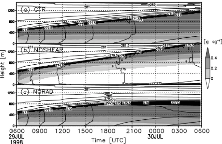
Figure 7a shows the time–height cross-sections of potential temperature and LWC for the CTR case. The boundary layer developed over a depth from 500 to 1200 m during 24 h, while the potential temperature in the layer gradually decreased from 273 to 271 K due to the surface and cloud-top cooling. The layer is always completely filled with clouds. During the last 3 h, the stratification near the surface became more stable with an increase in LWC.
Figure 8 shows the time–height cross-section of each TKE budget term for the CTR case (S, shear production; B, buoyancy production; T, transport; and D, dissipation). The TKE structure can be divided into two stages: the first is a developing stage with a cloud-filled boundary layer. Near the sur-face, the balance of TKE results from a balance between shear production (gain) and dissipation (loss) with smaller contributions from buoyancy (loss).
Figure 7. Time–height cross-sections of potential temperature (solid line) and LWC (grey area) for each case.
Below the cloud top, on the other hand, buoyancy (gain) from radiative cooling balances dissipation (loss). The TKE produced near the surface and cloud top is transported into the middle layer. The TKE budget during the developing stage can be summarized as follows: the shear-driven boundary layer and cloud-topped elevated mixed layer are coupled by transporting TKE into the middle layer.
The second stage is a mature stage characterized by decreasing production by shear near the surface, and buoyancy at the cloud top. Unlike the developing stage, there is no net transport of TKE into the middle layer, suggesting that the structure of the boundary layer is essentially decoupled between the shear-driven layer and cloud-topped mixed layer. Boundary-layer development has been essentially completed.
4.3. MECHANISM OF CLOUDLAYERING
For the formation of multiple cloud layers, two sources of TKE production are fundamentally important. Strong shear production over the ice surface potentially induces a single cloud layer through shear mixing under the negative buoyant production near the surface. This process occurs during the low-level cloud formation after a cyclonic event. Figure 9a compares TKE budget profiles from the CTR case after 24 h and the observational results. Although the CTR case and observations differ in terms of the number of cloud layers and the height of the boundary layer as well as the heteroge-neous surface condition, inducing the large deviation of the TKE budget terms near the surface as shown in Figure 5c, the modelled TKE structure is Figure 8. Time–height cross-section of each TKE budget term in the CTR case (S: shear production; B, buoyancy; T, transport; and D, dissipation).
similar to the observed structure below the 500-m level. This means that the lower part of the boundary layer is principally maintained under conditions of strong wind shear.
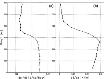
The second source of TKE production is radiative cooling at the cloud top, which modulates the evolution of the boundary layer after the formation of low-level cloud. In the NOSHEAR case, the boundary-layer clouds above a cloud free layer developed at higher levels (between heights of 500 and 1500 m) than that in the CTR (Figure 7b). These results mean that radiative cooling at the cloud top is important only for the development of the boundary layer. However, as the boundary layer develops, the cooled air is not transported towards the lower level in which the shear mixing occurs, suggesting that the amount of condensation will decrease. Figure 10 shows the vertical distributions of tendencies of liquid cloud and static stability for the CTR case after 24 h. The amount of cloud increases in the stable layer below 300 m and decreases in the neutral layer, which will divide the layer into cloud and cloud-free layers.
From the viewpoint of the observational results, the NORAD case can be considered as the case in which the upper cloud layer is advected over the existing lower cloud layer. The TKE profile of the NORAD is also similar to that in the observations (Figure 9b). Although the boundary layer is filled with cloud below the 800-m level, the production of TKE is limited below the 200-m level, which causes a more strongly stratified surface layer with an increase of LWC (Figure 7c). Comparing TKE profiles between the CTR and NORAD cases, the boundary-layer clouds tend to be separated in space
(a) CTR (b) NORAD
Figure 9. TKE budget for (a) CTR and (b) NORAD experiments after 24 h. Thick line, TKE production; thin line, buoyant term; dashed line, dissipation term. Observational results are also depicted by + (production), * (buoyancy), and(imbalance).
whether there is strong cloud-topped cooling or not (i.e., whether or not there is upper level cloud). This may be one of the reasons that cloud layering occurs frequently during the Arctic summer.
In the NOSHEAR case a cloud-topped boundary layer develops above a cloud-free layer higher than in the CTR case. The NOSHEAR case (Figure 7b) can be considered to be a special case for which the cloud-free layer appears through decoupling of TKE (in the absence of low-level cloud). In the NORAD case the development of the boundary layer ceased after the radiative process was removed (Figure 7c). Therefore, the decoupling of TKE signifies the beginning of cloud layering.
In this study, the effects of large-scale vertical motions and precipitation are not included in our LES model. Investigating the effects of radiation, large-scale vertical motion and drizzle, McInnes and Curry (1995) showed that radiative cooling under weak rising vertical motion was the most favourable situation for the maintenance of the multiple cloud layers. The effect of drizzle on the cloud layering was small unless rising vertical motion was absent. The remarkable contrast between their buoyantly driven, and our storm-driven, boundary layers is due to the existence of a thick mixing shear layer (200–300 m) that is comparable with that of the buoyantly mixed layer near the cloud top (Figure 8). Another factor for the cloud layering is the absorption of solar radiation in the middle part of the cloud layer, which separates into two layers by the local evaporation (Herman and Goody, 1976). Further, the change in the local surface condition due to solar radi-ation may affect the boundary-layer structure.
(a) (b)
Figure 10. Vertical distributions of (a) time change of liquid cloud and (b) static stability for the CTR after 24 h of simulation.
However, as long as the stormy conditions persist, the coupling between the shear-driven and buoyantly driven layers is strong enough to maintain the low-level cloud without large-scale vertical motions and/or solar radiative effects. Once the wind shear weakens, the boundary layer shifts to a buoy-antly driven system with a cloud-free layer (Figure 7b). If more upper cloud is advected, the boundary layer shifts to a shear-driven system (Figure 7c). Observations show that the lower cloud can persist for more than 3 h as a shear-driven boundary layer (Figure 3). The storm-driven cloudy boundary layer as a whole can be regarded as a long-lived system.
5. Concluding Remarks
Arctic stratus clouds under stormy conditions were investigated using aircraft observations and LES results for the case of 29 July 1998 during the SHEBA field program. Following the passing of a frontal system, a shallow cloud layer formed over the ice surface. Aircraft observations were carried out when the upper level cloud associated with a subsequent synoptic frontal system advected over the existing cloud layer, and showed that the TKE structure of the lower cloud layer was maintained by strong shear production within the lower part of the layer (below 200 m). In the upper part of the layer from 200 to 500 m, the production of TKE by shear and buoyancy was insignificant. The profiles of longwave radiation and heating rate based on the observations showed that downward longwave radiation emitted from the upper cloud suppresses the radiative cooling and resultant turbulent mixing in the lower cloud.
Three LES experiments were conducted to study the physical processes within the stormy cloudy boundary layer in detail. The control case showed that a cloud-filled boundary layer developed between heights of 500 and 1200 m. However, in the case without wind shear, a cloud-topped boundary layer with a cloud-free layer developed higher than the control case between heights of 500 to 1500 m, while in the simulation without radiative processes after 12 h of the control case, the development of a cloud-filled boundary layer was suppressed. Comparing the TKE structures from the three exper-iments, shear production near the surface under a negative buoyancy flux potentially has the effect of maintaining the low-level cloud and increasing the layer stability, while mixing by radiatively cooled air at the cloud top promotes the vertical condensational growth.
Once the cloud forms by shear mixing associated with cooling near the ice surface, the cloud-topped mixed layer gradually develops by radiative cooling (e.g., the control case). The production of TKE in the developing stage is coupled between the shear-mixed layer and cloud-topped mixed layer through TKE transport into the middle layer. However, once the cloud
reaches a certain height, dependent on the amount of cloud-top cooling, the two sources of TKE production begin to separate in space because insuffi-cient TKE is transported into the middle layer. Reduced transport of the cooled air into the middle layer causes less condensation, producing a cloud-free layer dividing lower and upper cloud layers. This self-decoupling of TKE is one possible mechanism for cloud layering under stormy conditions.
Another feature of the storm-driven cloudy boundary layer is that the low-level cloud persists under strong wind shear conditions near the surface even if an upper layer cloud associated with a cyclone is advected above. The TKE structure of our simulation without radiative cooling has the same charac-teristics as the observations, with strong shear production occurring in the lower half of the cloud layer and weak buoyancy in the upper half of the layer. This means that the existence of the lower cloud layer is prevented from further development and is maintained only in regions of shear mixing. This case is consistent with the prevailing conditions in June and July over the Arctic Ocean, the only two months when multiple cloud layers are ob-served more frequently than a single cloud layer.
Acknowledgements
This research was supported by the NSF SHEBA program and the DOE ARM program. We would like to thank Dr. J.O. Pinto for providing us with the algorithm to process the C-130 turbulent data. The NCEP/NCAR rea-nalyses were obtained from the archive at NCAR. We would like to express our thanks to Gayle Sugiyama for her careful reading of the manuscript and valuable suggestions. Part of this work was performed under the auspices of the U.S. Department of Energy by University of California, Lawrence Liv-ermore National Laboratory under Contract W-7405-Eng-48.
References
Andren, A.: 1995, ‘The Structure of Stable Stratified Atmospheric Boundary Layers: A Large-Eddy Simulation Study’,Quart. J. Roy. Meteorol. Soc.121, 961–985.
Bromwich, D. H., Tzeng, R. -Y., and Parish, T. R.: 1994, ‘Simulation of the Modern Arctic Climate by the NCAR CCM1’,J. Climate7, 1050–1069; 715–746.
Bru¨mmer, B., Busack, B., and Hoeber, H.: 1994, ‘Boundary-Layer Observations over Water and Arctic Sea-Ice during On-Ice Air Flow’,Boundary-Layer Meteorol.68, 75–108. Curry, J. A., Ebert, E. E., and Herman, G. F.: 1988, ‘Mean and Turbulent Structure of
Summer Time Arctic Cloudy Boundary Layer’,Quart. J. Roy. Meteorol. Soc. 114, 715– 746.
Curry, J. A., Rossow, W. B., Randall, D., and Schramm, J. L.: 1996, ‘Overview of Arctic Cloud and Radiation Characteristics’,J. Climate9, 1731–1764.
Curry, J. A. and 26 Coauthors: 2000, ‘FIRE Arctic Clouds Experiment’,Bull. Am. Meteorol. Soc.81, 5–29.
Curry, J. A., Schramm, J. L., Alam, A., Reeder, R., Arbetter, T. E., and Guest, P.: 2002, ‘Evaluation of Data Sets Used to Force Sea Ice Models in the Arctic Ocean’,J. Geophys. Res.107, doi:10.1029/2000JC000466.
Herman, G. F. and Curry, J. A.: 1984, ‘Observational and Theoretical Studies of Solar Radiation in Arctic Stratus Clouds’,J. Climate Appl. Meteorol.23, 5–24.
Herman, G. F. and Goody, R.: 1976, ‘Formation and Persistence of Summertime Arctic Stratus Clouds’,J. Atmos. Sci.54, 2799–2812.
Intrieri, J. M., Shupe, M. D., Uttal, T., and McCarty, B. J.: 2002, ‘An Annual Cycle of Arctic Cloud Characteristics Observed by Radar and Lidar at SHEBA’,J. Geophys. Res. 107, 8030, doi:10.1029/2000JC000432.
Key, J.: 2001, Streamer User’s Guide, Cooperative Institute for Meteorological Satellite Studies, University of Wisconsin, 96 pp.
Klemp, J. B. and Duran, D. R.: 1983, ‘An Upper Boundary Condition Permitting Internal Gravity Wave Radiation in Numerical Meso-Scale Models’,Mon. Wea. Rev.111, 430–444. Kosovic´, B.: 1997, ‘Subgrid-Scale Modeling for the Large-Eddy Simulation of
High-Reynolds-Number Boundary Layers’,J. Fluid Mech.336, 151–182.
Kosovic´, B. and Curry, J. A.: 2000, ‘A Large Eddy Simulation Study of a Quasi-Steady, Stably Stratified Atmospheric Boundary Layer’,J. Atmos. Sci.57, 1052–1068.
Lawson, R. P., Baker, B. A., Schmitt, C. G., and Jensen, T. L.: 2001, ‘An Overview of Microphysical Properties of Arctic Clouds Observed in May and July 1998 during FIRE ACE’,J. Geophys. Res.106, 14989–15014.
Mason, P. J. and Derbyshire, S. H.: 1990, ‘Large-Eddy Simulation of the Stably-Stratified Atmospheric Boundary Layer’,Boundary-Layer Meteorol.42, 117–162.
Maykut, G. A. and Untersteiner, N.: 1971, ‘Some Results from a Time-Dependent Thermo-dynamic Model of Sea Ice’,J. Geophys. Res.,76, 1550–1575.
McInnes, K. and Curry, J. A.: 1995, ‘Modeling the Mean and Turbulent Structure of the Summertime Arctic Cloudy Boundary Layer’,Boundary-Layer Meteorol.73, 125–143. Nicholls, S.: 1984, ‘The Dynamics of Stratocumulus: Aircraft Observations and Comparisons
with a Mixed Layer Model’,Quart. J. Roy. Meteorol. Soc.110, 783–820.
Nicholls, S. and Leighton, J.: 1986, ‘An Observational Study of the Structure of Stratiform Cloud Sheets: Part I. Structure’,Quart. J. Roy. Meteorol. Soc.112, 431–460.
Otte, M. J. and Wyngaard, J. C.: 2001, ‘Stably Stratified Interfacial-Layer Turbulence from Large Eddy Simulations’,J. Atmos. Sci.58, 3424–3442.
Perovich, D. K. and 22 Coauthors: 1999, ‘Year on Ice Gives Climate Insights’,EOS,Trans. Am. Geophys. Union80, 481–486.
Persson, P. O. G., Fairall, C. W., Andreas, E. L., Guest, P. S., and Perovich, D. K.: 2002, ‘Measurements near the Atmospheric Surface Flux Group Tower at SHEBA: Near-Surface
Conditions and Surface Energy Budget’, J. Geophys. Res. 107, 8045, doi:10.1029/
2000JC000705.
Pinto, J. O.: 1998, ‘Autumnal Mixed-Phase Cloudy Boundary Layers in the Arctic’,J. Atmos. Sci.55, 2016–2038.
Ruffieux, D. R., Persson, P. O. G., Fairall, C. W., and Wolfe, D. E.: 1995, ‘Ice Pack and Lead Surface Energy Budgets during LEADEX 92’,J. Geophys. Res.100, 4593–4612.
Saiki, E. M., Moeng, C. -H., and Sullivan, P. P.: 2000, ‘Large-Eddy Simulation of the Stably Stratified Planetary Boundary Layer’,Boundary-Layer Meteorol.95, 1–30.
Shupe, M. D., Uttal, T., Matrosov, S. Y., and Frisch, A. S.: 2001, ‘Cloud Water Contents and Hydrometeor Sizes during the FIRE Arctic Clouds Experiment’, J. Geophys. Res. 106, 15015–15028.
Uttal, T. and 27 Coauthors: 2002, ‘Surface Heat Budget of the Arctic Ocean’, Bull. Amer. Meteorol. Soc.83, 255–275.